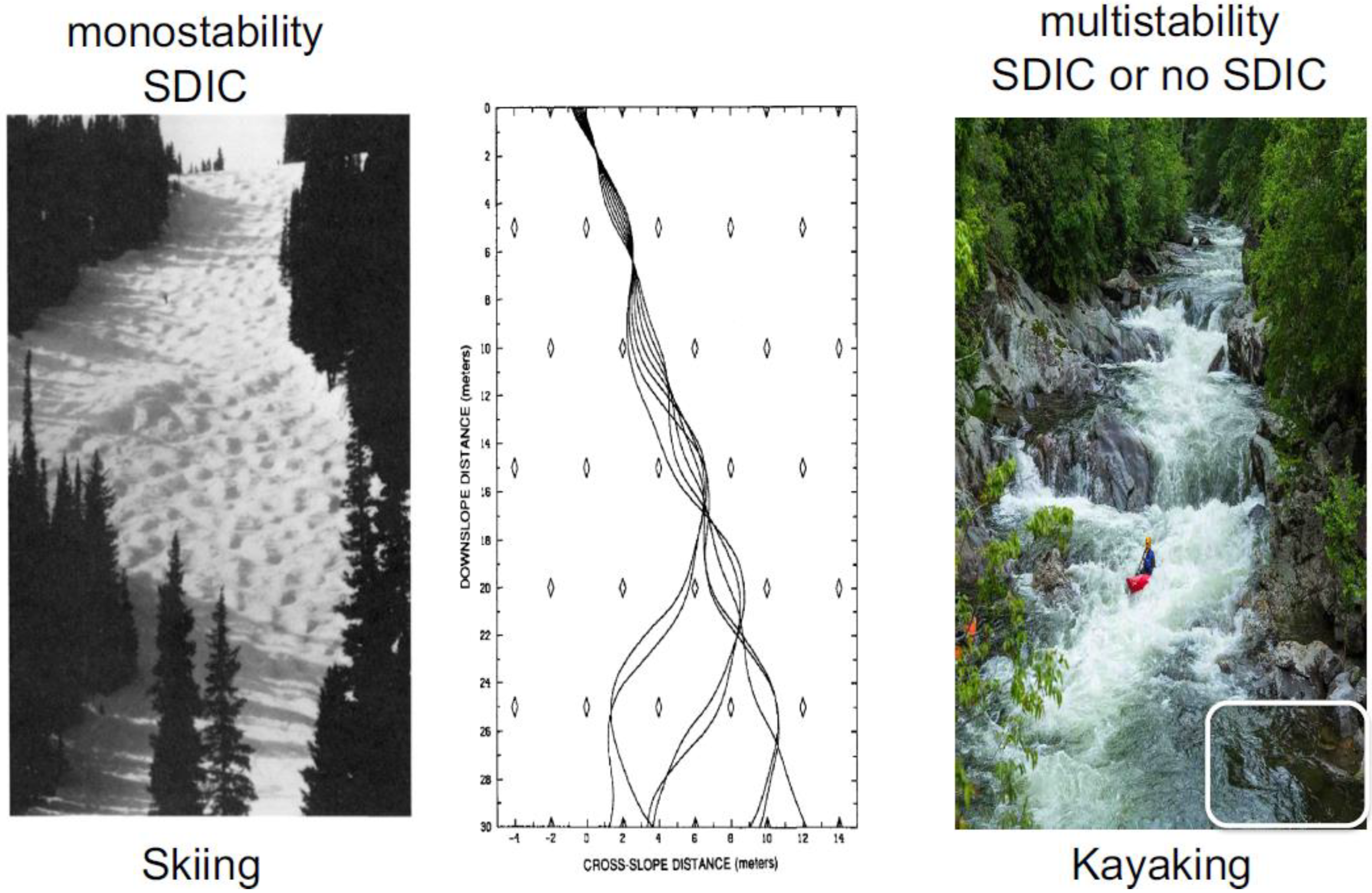
1. An Analogy for Monostability and Multistability Using Skiing and Kayaking
To help readers, the sensitive dependence of solutions on initial conditions (SDIC)
[1][2], monostability, and multistability, which are the most important concepts regarding predictability studies, are first illustrated using real-world analogies of skiing and kayaking. To explain SDIC, the book entitled “The Essence of Chaos” by Lorenz, 1993
[1] applied the activity of skiing (left in
Figure 1) and developed an idealized skiing model for revealing the sensitivity of time-varying paths to initial positions (middle in
Figure 1). Based on the left panel, when slopes are steep everywhere, SDIC always appears. This feature with a single type of solution is referred to as monostability.
In comparison, the right panel of
Figure 1 for kayaking is used to illustrate multistability. In the photo, the appearance of strong currents and a stagnant area (outlined with a white box) suggests instability and local stability, respectively. As a result, when two kayaks move along strong currents, their paths display SDIC. On the other hand, when two kayaks move into a stagnant area, they become trapped, showing no typical SDIC (although a chaotic transient may occur
[3]). Such features of SDIC or no SDIC suggest two types of solutions and illustrate the nature of multistability.
2. The Generalized Lorenz Model (GLM) and The Lorenz 1963 (L63) Model
Over the past several years, a series of papers regarding high-dimensional Lorenz models that have applied a different number of Fourier modes have yielded the following generalized Lorenz model (GLM)[4][5]:
Here, τ is dimensionless time. The three integers j, M, and N are related to the number of additional Fourier modes within higher dimensional Lorenz models (LMs). While M represents the total number of modes (or equations), N indicates the total number of pairs for higher wavenumber modes that do not appear within the original L63 Model. The time-independent parameters, including σ and r, represent the Prandtl number and the normalized Rayleigh number (or the heating parameter), respectively. The heating parameter represents a measure of temperature differences between the bottom and top layers. Parameter “a” is defined as the ratio of the vertical scale of the convection cell to its horizontal scale and a2 = 1/2. The last three parameters in Eq. (6) are coefficients for the dissipative terms. Detailed discussions for each of the above terms can be found in the 2-page Supplementary Materials of Shen et al., 2021[5]. Variable X denotes the amplitude of the Fourier mode for the stream function. Variables (Y, Z), (Y1, Z1), (Y2, Z2), and (Y3, Z3) are referred to as the primary, secondary, tertiary, and quaternary modes, respectively, and represent the amplitudes of the Fourier modes at different wave numbers for temperature. The GLM with M = 5, 7, or 9 is referred to as the 5D-, 7D-, or 9DLM, respectively, and the classical L63 model (referred to as the 3DLM) can be obtained using Eqs. (1-3) without the nonlinear term XY1, written as follows [2]:
This research keeps σ = 10 and b = 8/3, but varies r in different runs.
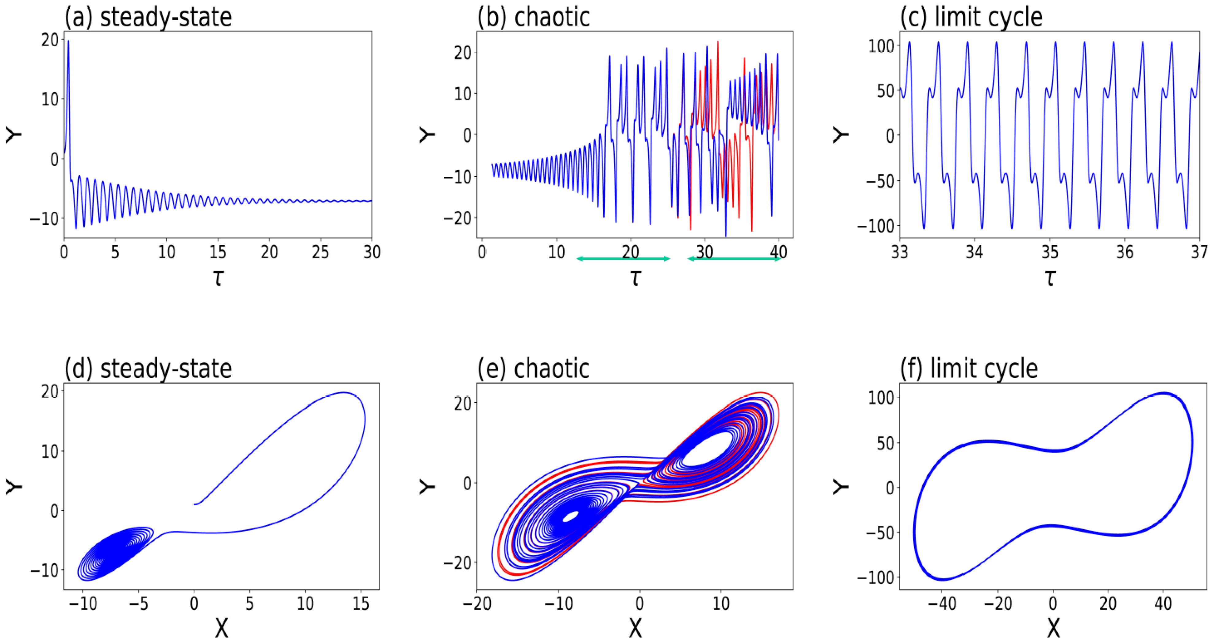
3. Single-Types of Attractors and Monostability within the L63 Model
Previous studies have shown that the L63 model produces three types of solutions at small, medium, and large heating parameters
[5][6][7]. Below, three numerical experiments, which apply three different values of Rayleigh parameters and keep the other two parameters as constants within the same L63 model, are discussed. The selected values of the Rayleigh parameters are 20, 28, and 350, representing weak, medium, and strong heating, respectively. For each of the three cases, both control and parallel runs were performed. The only difference in the two runs was that a tiny perturbation with
ϵ = 10−10 was added into the initial condition (IC) of the parallel run. The SDIC along with continuous dependence of solutions on IC (CDIC) is then discussed. Solutions of the
Y component are provided in the top panels of
Figure 2. Three panels, from left to right, display long-term time independent responses, irregular temporal variations, and regular temporal oscillations referred to as steady-state, chaotic, and limit cycle solutions, respectively. Corresponding solutions within the
X-Y phase space are shown in the bottom panels of
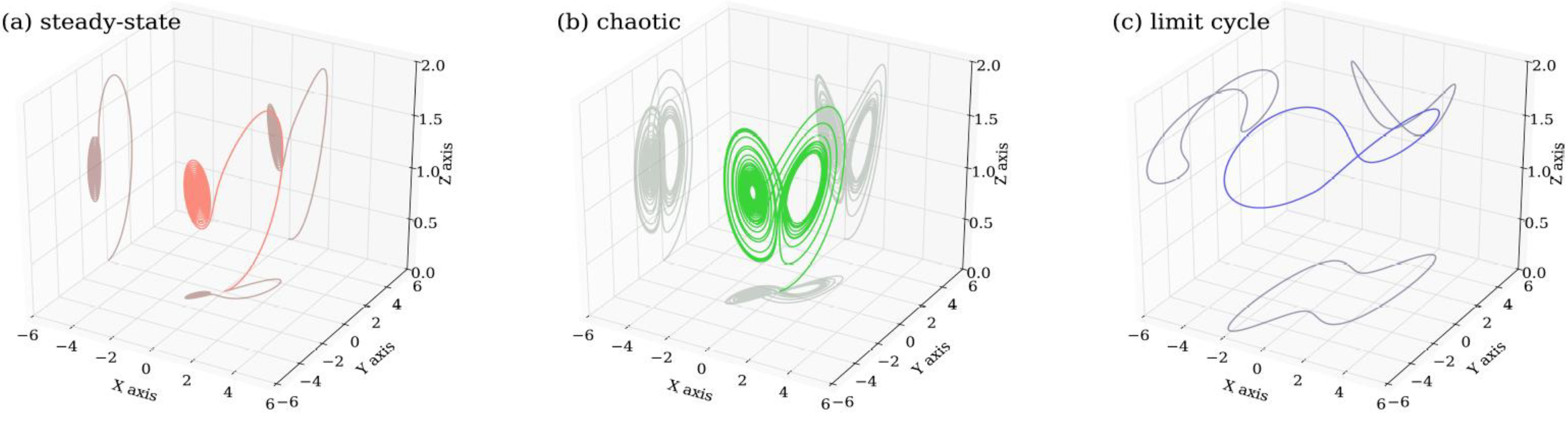
Figure 2. Non-chaotic, steady-state and limit cycle solutions become point attractors and periodic attractors in panels 2d and 2f, respectively. As a comparison, all three types of attractors within the three-dimensional
X-Y-Z phase space are provided in
Figure 3. Below, the features of SDIC for chaotic solutions are further discussed.
Figure 2. Three types of solutions within the Lorenz 1963 model. Steady-state (
a,
d), chaotic (
b,
e), and limit cycle (
c,
f) solutions appear at small, moderate, and large normalized Rayleigh parameters (i.e.,
r = 20, 28, and 350), respectively. Control and parallel runs are shown in red and blue, respectively. SDIC is indicated by visible blue and red curves in panel (
b), where the first and second green horizontal lines indicate CDIC and SDIC, respectively. (
a–
c) depict the time evolution of
Y. (
d–
f) show orbits within the
X–
Y space, appearing as a point attractor (
a,
d), a chaotic attractor (
b,
e), and a periodic attractor (
c,
f), respectively (after Shen et al., 2021
[6]). The other two parameters are kept as constants: σ = 10 and b = 8/3. The initial conditions of
(X, Y, Z) for the control and parallel runs are
(0,1,0) and
(0, 1 + ϵ, 0), respectively.
Figure 3. Three types of solutions within the X–Y–Z phase space obtained from the Lorenz 1963 model. Panels (a–c) display a steady-state solution, a chaotic solution, and a limit cycle with small, medium, and large heating parameters, respectively. While panels (a,b) show the solution for τ ∈ [0, 30], to reveal its isolated feature, panel (c) displays the limit cycle solution for τ ∈ [10, 30]. Values of parameters are the same as those in the control run in Figure 2.
For chaotic solutions in the middle panels of Figure 2, both the control and parallel runs produced very close responses at an initial stage, but very different results at a later time. Initial comparable results indicate that CDIC is an important feature of dynamical systems. Despite initial tiny differences, large differences at a later time, as indicated by the red and blue curves in Figure 2b, revealed the feature of SDIC. Such a feature suggests that a tiny change in an IC will eventually lead to a very different time evolution for a solution. However, the concept of SDIC does not suggest a causality relationship. Specifically, the initial tiny perturbation should not be viewed as the cause for a specific event (e.g., a maximum or minimum) that subsequently appears or for any transition between different events.
As discussed above, depending on the relative strength of the heating parameter, one and only one type of steady-state, chaotic, and limit cycle solution appears within the L63 model. Such a feature is referred to as monostability, as compared to multistability for coexisting attractors. Over several decades, chaotic solutions and monostability have been a focal point, yielding the statement “weather is chaotic”. As discussed below, such an exclusive statement is being revised by taking coexisting attractors and time varying multistability into consideration.
4. Coexisting Attractors and Multistability within the Generalized Lorenz Model
Based on various high-dimensional Lorenz models
[8][9][10][11], a generalized multi-dimensional Lorenz model (GLM) has been developed
[4][7][12]. Mathematical descriptions of the GLM are summarized in the Supplementary Materials of Shen et al., 2021
[5]. Major features of the GLM include: (1) any odd number of state variables greater than three; (2) the aforementioned three types of solutions; (3) hierarchical spatial scale dependence (e.g.,
[10][11]); and (4) two kinds of attractor coexistence
[4][5][12][13]. Additionally, aggregated negative feedback appears within high-dimensional LMs when the negative feedback of various smaller scale modes is accumulated to provide stronger dissipations, requiring stronger heating for the onset of chaos in higher-dimensional LMs. Such a finding is indicated in Table 2 of Shen, 2019
[7], which compared the critical values of heating parameters for the onset of chaos within the L63 and GLM that contains 5
–9 state variables. Sufficiently large, aggregated negative feedback may cause (some) unstable equilibrium points to become stable and, thus, enable the coexistence of stable and unstable equilibrium points, yielding attractor coexistence, as illustrated below using the GLM with nine state variables.
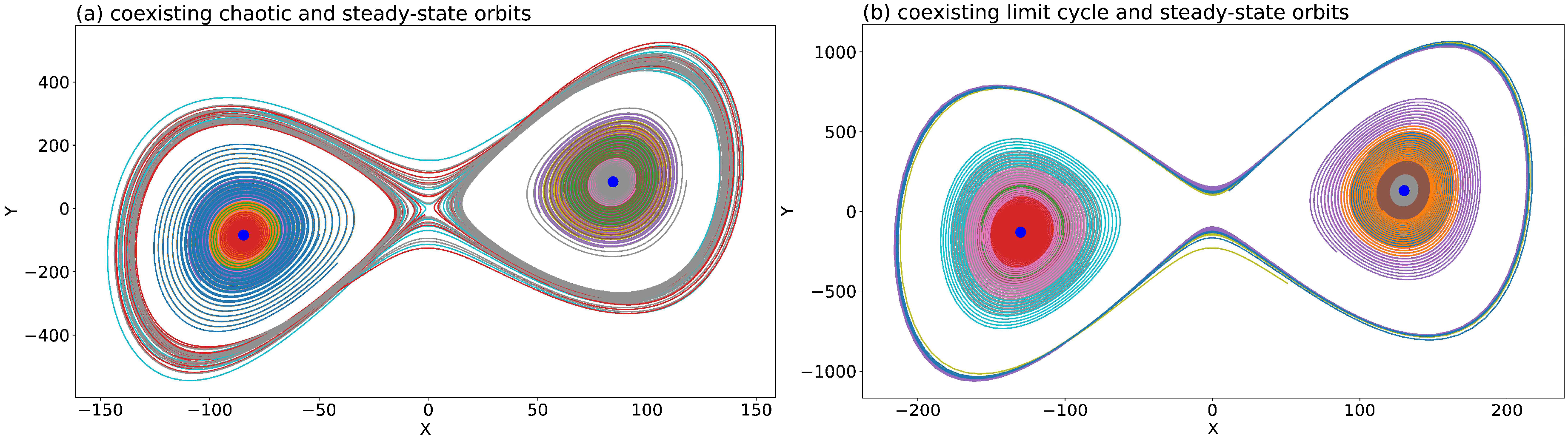
Amongst the three types of solutions (i.e., steady-state, chaotic, and limit-cycle solutions), two types of solutions may appear within the same model that applies the same model parameters but different initial conditions. Such a feature is known as attractor coexistence. The GLM produces two kinds of attractor coexistence, including coexisting chaotic and steady-state solutions and coexisting limit-cycle and steady-state solutions, referred to as the 1st and 2nd kinds of attractor coexistence, respectively. To illustrate coexisting attractors that display a dependence on initial conditions,
Figure 4 displays two ensemble runs, each run using 128 different initial conditions that were distributed over a hypersphere (e.g., Shen et al., 2019
[12]). The 1st and 2nd kinds of attractor coexistence are illustrated using values of 680 and 1600 for the heating parameter, respectively. As shown in
Figure 4a, 128 orbits with different starting locations eventually reveal the 1st kind of attractor coexistence for one chaotic attractor, and two point attractors. As clearly seen in
Figure 4a, each of the chaotic and non-chaotic attractors occupies a different portion of the phase space. By comparison, in
Figure 4b, 128 ensemble members produce the 2nd kind of attractor coexistence, consisting of limit cycle and steady-state solutions.
Figure 4. Two kinds of attractor coexistence using the GLM with 9 modes. Each panel displays orbits from 128 runs with different ICs for τ ∈ [0.625, 5]. Curves in different colors indicate orbits with different initial conditions. (a) displays the coexistence of chaotic and steady-state solutions with r = 680. Stable critical points are shown with large blue dots. (b) displays the coexistence of the limit cycle and steady-state solutions with r = 1600.
The above two kinds of attractor coexistence occur in association with the coexistence of unstable (i.e., a saddle point) and stable equilibrium points. As discussed in Shen, 2019
[4], the appearance of local stable equilibrium points is enabled by the so-called aggregated negative feedback of small-scale convective processes. The feature with coexisting attractors is referred to as multistability, as compared to monostability for single type attractors. As a result of multistability, SDIC does not always appear. Namely, SDIC appears when two orbits become the chaotic attractor that occupies one portion of the phase space; it does not appear when two orbits move towards the same point attractor that occupies the other portion of the phase space.
In a recent study by Shen et al.
[14], three major kinds of butterfly effects can be identified: (1) SDIC, (2) the ability of a tiny perturbation in creating an organized circulation at a large distance, and (3) the hypothetical role of small scale processes in contributing to finite predictability. While the first kind of butterfly effect with SDIC is well accepted, the concept of multistability suggests that the first kind of butterfly effect does not always appear.
5. Time Varying Multistability and Recurrent Slowly Varying Solutions
Within Lorenz models, a time varying heating function may be applied to represent a large-scale forcing system
[5][15]; and references therein). Since the heating function changes with time, the first and second kinds of attractor coexistence alternatively appear, leading to time varying multistability and transitions from chaotic to non-chaotic solutions. An analysis of the above two features can help reveal the predictable nature of recurrence for slowly varying solutions, and a less predictable (or unpredictable) nature for the onset for emerging solutions (defined as the exact timing for the transition from a chaotic solution to a non-chaotic limit cycle type solution).
Here, by extending the study of Shen et al., 2021
[5], the GLM with a time-dependent heating function is applied in order to revisit time varying multistability.
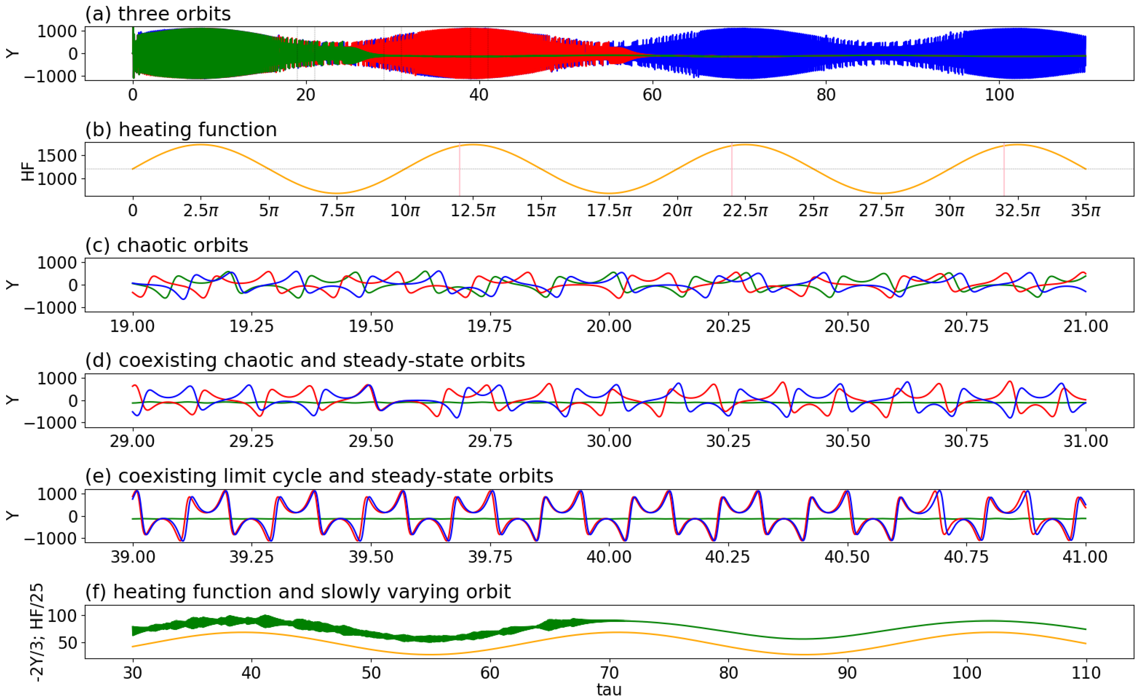
Figure 5a displays three trajectories during a dimensionless time
τ between 0 and 35
π (i.e.,
τ ∈ [0, 35π]). As shown in the second panel of
Figure 5, these solutions were obtained using tiny differences in ICs and a time varying Rayleigh parameter. The 3rd to 5th panels display the feature of SDIC
[1][2][14][16], the first kind of attractor coexistence (i.e., coexisting steady-state and chaotic solutions), and the second kind of attractor coexistence (i.e., coexisting steady-state and periodic solutions) at different time intervals, respectively. The alternative appearance of two kinds of attractor coexistence suggests time varying multistability. By comparison, the 6th panel indicates that once a “steady state” solution appears (when local time changes for all state variables become zero), it remains “steady” and slowly varies with the time-dependent heating function. Such a recurrent, slowly varying solution may, in reality, be used as an analogy for recurrent seasons.
Figure 5. Two kinds of attractor coexistence revealed by three trajectories using a time varying heating parameter (i.e., Rayleigh parameter),
r = 1200 + 520 sin (τ/5), within a GLM (Shen, 2019
[4]). The green, blue, and red lines represent the solutions of the control and two parallel runs. The parallel runs include an initial tiny perturbation,
ϵ = 10−8 or
ϵ = −10−8. The heating function is indicated by an orange line. From top to bottom, panels (
a,
b) display the three orbits and the heating parameters for τ
∈ [0, 35π], respectively. Panel (
c) for τ
∈ [19, 21] displays diverged trajectories, showing SDIC. The first kind of attractor coexistence (i.e., coexisting chaotic and steady-state solutions) is shown in panel (
d) for τ
∈ [29, 31]. The green line, indeed, represents a steady state solution. The second kind of attractor coexistence (i.e., coexisting regular oscillations and steady-state solutions) is shown in panel (
e) for τ
∈ [39, 41]. Panel (
f) displays a nearly steady-state solution (2Y/3) and the heating function for τ
∈ [30, 110]. The three vertical lines in panel (
b) indicate the starting time for the analysis in
Figure 6. (After Shen et al., 2021
[5]).
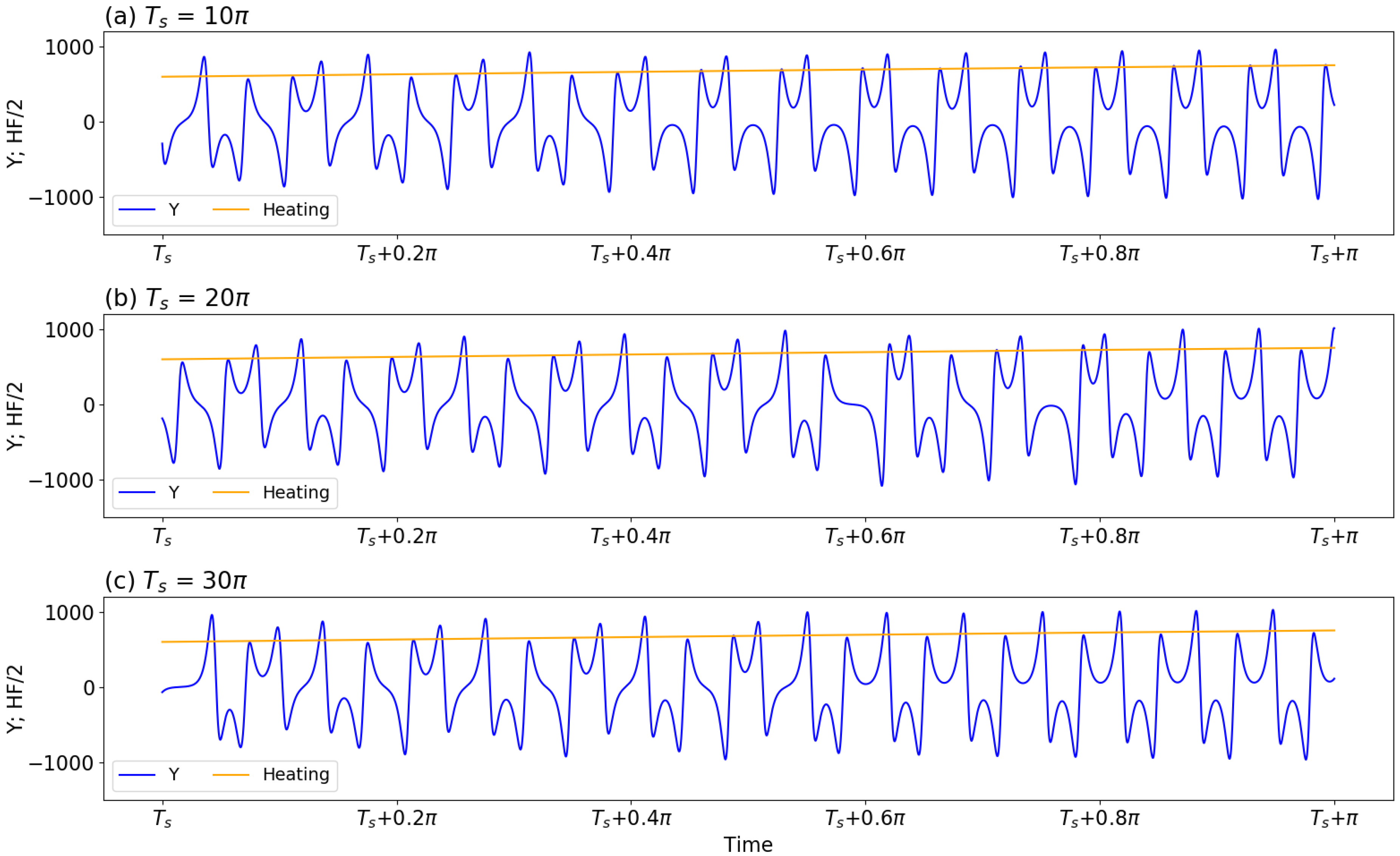
Figure 6. Panels (a–c) display the same trajectory during three different time intervals of τ ∈ [Ts, Ts + π], with the starting time Ts equal to 10π, 20π, and 30π, respectively. The orange line in each panel represents the half value of the heating function.
6. Onset of Emerging Solutions
Although the GLM with a time dependent heating function produces time varying multistability, as a result of simplicity within the model and the complexity of the problem, here, no attempt is made to address the attractor basin, intra-transitivity, final state sensitivity, or a hidden attractor (e.g.,
[5][13]). Instead, the transition from one type of solution to the other type of solution is a focus. Here, for emulating a real-world scenario for the first appearance of African Easterly waves during a seasonal transition
[5][7], the transition from a chaotic (irregular) solution to a limit cycle type (regular) solution is analyzed. Within
Figure 5, while two trajectories display a sensitivity to initial conditions after
τ > 19 (
Figure 5c), they become regularly oscillatory solutions with comparable frequencies and amplitudes for
τ ∈ [39, 41] (
Figure 5e). Reappearance of the regular solution (i.e., limit cycle type solutions) is defined as the “onset of an emerging solution”. Below, a challenge in predicting the onset of the transition from a chaotic solution to a regularly oscillatory solution is illustrated.
Figure 6 displays the same trajectory during three different time intervals of τ ∈ [Ts, Ts + π]. Here, the starting time Ts is equal to 10π, 20π, and 30π in panels (a)–(c), respectively. An orange line in each panel represents the half value of the heating function. Given any vertical line, its intersection with each of the three orange lines in all panels yields the same value for the heating parameter. In other words, although the starting time is different, the time evolution for the heating functions is exactly the same in all three panels. As a result, if the appearance of regularly oscillatory solutions is solely determined by the values of the heating function, the same time evolution of oscillatory solutions should appear in the three panels of Figure 6. However, differences are observed. For example, panel (a) displays the onset of a regularly oscillatory solution (e.g., the timing of the regular solution) at τ = Ts + 0.4π = 10.4π. Panels (b) and (c) show an onset around Ts + 0.8π = 20.8π and Ts + 0.6π = 30.6π, respectively. As a result of the time lag, the correlation coefficient for the solution curves in any two panels is low, although the solutions are regularly oscillatory. The results not only indicate a challenge in predicting the onset of oscillatory solutions but also suggest the importance of removing phase differences for verification (to obtain a better correlation between two solution curves).
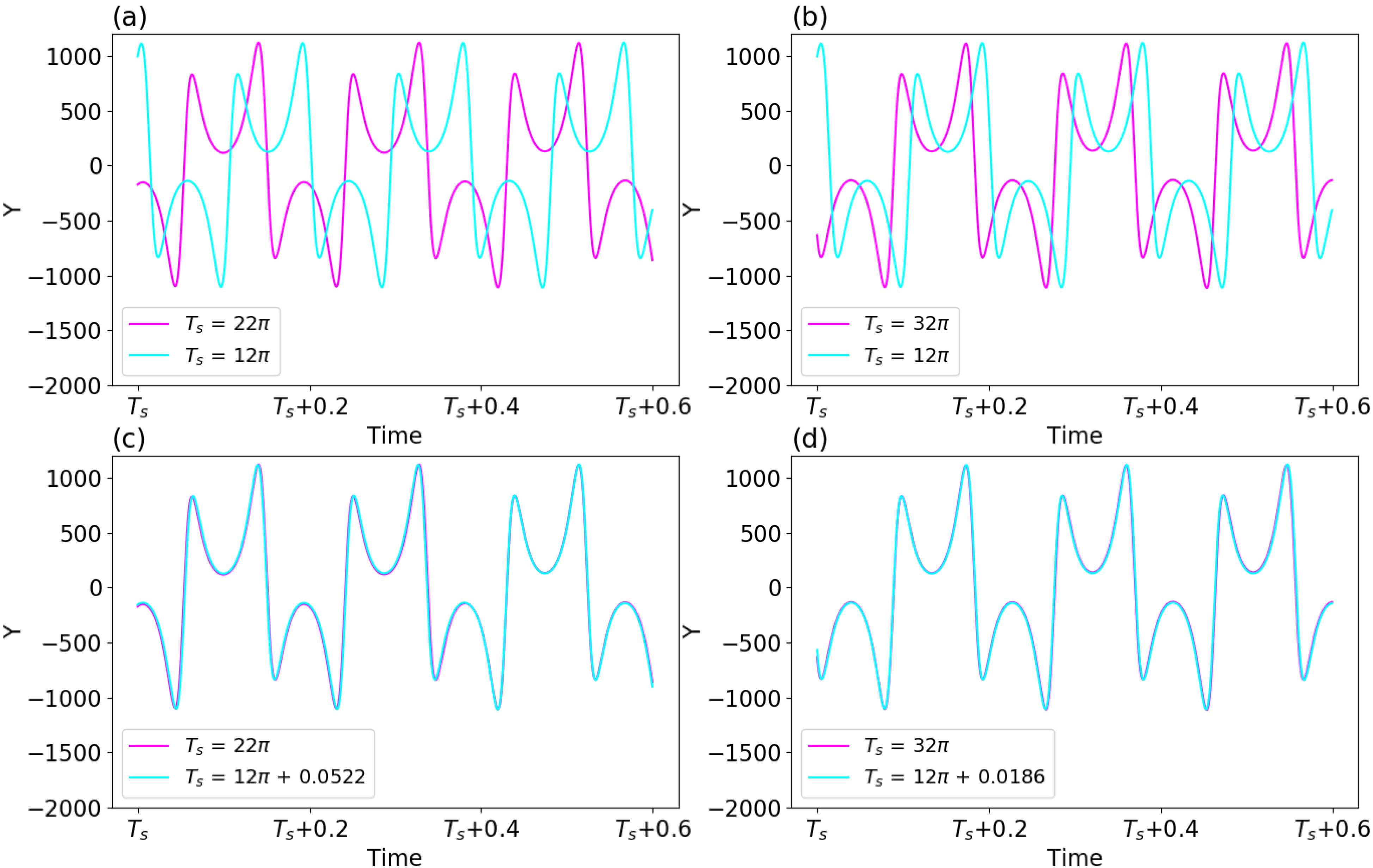
For the three solution curves (which represent the same trajectory at different time intervals) in Figure 6, different times for the onset of solutions suggest a time lag (or phase differences). However, the period and amplitude for solutions within the regime of limit-cycle solutions are comparable, suggesting an optimistic view in predictability. Similar to Figure 6, Figure 7a,b provides the same trajectory during three different time intervals of τ ∈ [Ts, Ts + π], including Ts for 12π, 22π, and 32π. Such a choice is required in order to assure the full development of nonlinear oscillatory solutions. The selected time intervals are referred to as Epoch-1, Epoch-2, and Epoch-3, respectively, and the solution curve from the first epoch (i.e., Epoch-1) is used as a reference curve. The top panels clearly show phase differences amongst the solution curves, although the heating function remains the same for selected epochs. For solution curves during two different epochs, their cross correlation is computed to determine a time lag. Such a time lag is then considered to have a different starting time for the first epoch. For example, in panel (c), a time lag of Δτ = 0.0522 is added to become a new starting time for the revised first epoch, referred to as a revised Epoch-1. After the time lag is considered, the solution curves for revised Epoch-1 and Epoch-2 are the same. In a similar manner, panel (d) displays the same evolution for solution curves for another revised Epoch-1 and Epoch-3.
Figure 7. Panels (a,b) display the same trajectory during three different time intervals of τ ∈ [Ts, Ts + π], with the starting time Ts equal to 12π, 22π, and 32π, respectively. These three time intervals are referred to as Epoch-1, Epoch-2, and Epoch-3, respectively. In panels (c,d), to adjust the phase differences between two solutions curves, a time lag is added into Epoch-1.
Time varying multistability associated with the alternative occurrence of two kinds of attractor coexistence yields the alternative and concurrent appearance of various types of solutions. Such a feature indicates complexities of weather and climate that possess both chaotic and non-chaotic solutions, and their transitions. While chaotic solutions and their transition to regular solutions possess limited predictability, slowly varying solutions and nonlinear oscillatory solutions (i.e., limit-cycle type solutions) may have better predictability. The onset of an emerging solution (i.e., during a transition from a chaotic solution to a limit-cycle type solution) suggests a different predictability problem. In summary, the above discussions of various types of solutions support the revised view that emphasizes the dual nature of chaos and order in weather and climate.
 +1 credit