Shape-from-Focus (SFF) methods have been developed for about twenty years - see ^[1] for the first publication. They able to obtain the shape of 3D objects from a series of partially focused images. It is based on discrete Fourier Transforms and Phase Correlation. Some statistical characterirstics are also used. 

1. Sharpness Zone

1.1 Focal Plane and Sharpness Zone 

In technical practice, the confocal microscope serves as a standard instrument imaging microscopic three-dimensional surfaces. It has a very small depth of the optical field with its advanced hardware being capable of removing non-sharp points from the images. The points of the object situated close to the focal plane can be seen as sharp points. The parts lying further above or beneath the focal plane (out of the sharpness zone) are invisible being represented as black regions if the confocal mode is on. In this way, a so-called optical cut is obtained. In the case of non-confocal (standard) mode, the areas lying outside the sharpness zone are displayed as blurred, as they would be with a standard camera. SSFs are able to identify these focused parts to compose a fully focused 2D image and to reconstruct a 3D profile of the surface to be observed ^[2]. 

1.2 Multifocal Image

To create a 2D or 3D reconstruction, it is necessary to obtain a series of images of an identical object, each of them with different focusing with each object point being focused in one of the images (in the ideal case) – this is referred to as a multifocal image. For the acquisition of a large multifocal image, the camera must be mounted on a stand so that it can be moved in the direction approximately orthogonal to the surface with a controlled step. Different transformation and different sharp parts must be identified and composed in a 2D or 3D model.

2. Mathematical Background of Image Registration

With a confocal microscope or CCD camera, we can assume that the field of view is small and the projection used is parallel. In this case, all images are provided in the field of view with identical sizes with the corresponding pixels having the identical coordinates in separate partial focused images. However, this assumption does not hold for larger samples; then, the angle of the projection lines is not negligible with the view fields (and the coordinates of the corresponding pixels) being clearly different for each image

Before reconstruction, all geometric transformations must be identified in the image series to be eliminated. Image processing requires the images transformed for the structures studied to be at the same position in all of them. Finding the transformation is done by image registration.A method suitable tool for this is the Fourier transform and phase correlation.

2.1. Discrete Two-Dimensional Fourier Transform

A discrete standard Fourier transform of a function

is the function

A discrete standard inverse Fourier transform of a function

is the function

2.2. Phase Correlation

The phase correlation has proved to be a powerful tool (not only) for the registration of particular focused images. For functions

, it is defined as 

with its modification being

where the bar denotes complex conjugation,

is a bounded real function such that

are  arbitrary constants and is multiplication of matrices element by element.

2.4. Distribution

A one-dimensional

-distribution is a limit of a function sequence

for which

and 

A two-dimensional case by analogy.

3. Identification of Transforms

3.1. Identical Images

Let be any real function. Then 

i.e.  the phase correlation of two identical images is equal to Dirac distribution.

3.2. Shifted Images

If two functions a re shifted in arguments, that is

their Fourier transforms are shifted in phase

with their phase-correlation function being the

-distribution shifted in arguments by the opposite shift vector

This is the principal idea of phase correlation. Using phase correlation, rather than finding a shift between two images, we can just find the only non-zero point in a matrix. If the images are not identical (up to a shift), i.e., if the images are not ideal, the phase-correlation function is more complex, but still has a global maximum at the point whose coordinates correspond to the shift vector.

3.3. Rotated Images

The phase-correlation function can also be used for estimating the image rotation and rescale. Let

be function rotated and shifted in arguments, i.e. 

Their Fourier spectra 

;  and amplitude spectra

;  are related as follows:

The shift results in a phase shift and the spectra are rotated the same way as the original functions. A crucial step here is the transformation of the amplitude spectra into polar coordinates to obtain functions

such that

. The rotation about an unknown centre has been transformed into a shift. This shift is estimated by the standard phase correlation (see the previous paragraph) after a reverse rotation by the angle measured, the shift

is then measured in another computation of the phase correlation.

3.4. Scaled Images 

Let be function rotated, shifted and scaled in arguments, i.e.

Their Fourier spectra and amplitude spectra are related as follows:

The shift results in a phase shift, the spectra are rotated the same way as the original functions and scaled with a reciprocal factor. A crucial step here is the transformation of the amplitude spectra into the logarithmic-polar coordinates

to obtain

such that

Both rotation and scale change have been transformed to a shift. The unknown angle

and unknown factor

can be estimated by means of the phase correlation applied to the amplitude spectra in the logarithmic-polar coordinates

. After reverse rotating function by the estimated angle and scaling by the factor , the shift vector

can be estimated by means of the standard phase correlation.

See ^[3] for more relevant information.

3.5. Multifocal Registration

Let

be the image series to be registered with image

acquired by means of the biggest angle of view. This image will be not transformed or (formally) it will be transformed by the identity mapping into the image

. Now we must find the transform  to obtain image which only differs from

in focussed and blured parts. In the same way, transforms

must be found.  

After multiplying both images

by the chosen window function, rotation angle and scale factor

will be determined by the method described in section 3. 4. Then, image

is rotated by the angle

and scaled by the factor

to compensate for the rotation and scale-change found by the phase correlation, creating image

. Between images and, only the shifted and different focused and blurred parts remain. Now we can apply phase correlation to find the shift

shifting image by the vector to compensate for the shift, creating image

which only differs from in the focused and blurred parts.  

More information is possible to find in ^{[4] [5]}. 

4. Focusing Criteria

The detectors of blurred areas (focusing criteria) can be based on different principles. We use cosine Fourier transform in suitable  neighbourhood of processed pixel. Whereas the low frequencies in the amplitude spectrum detect the blurred parts of the image, the very high ones only mean noise. Therefore, a suitable weight must be assigned to each frequency when the sharpness detector is calculated.

In our software, the following detectors may be used:

where

is the cosine spectrum of the pixel neighborhood,

 

5. 2D and 3D Reconstructions

A 2D reconstruction consists in composing a new image that contains only the focused parts of a registered multifocal image. The registration and detection of the focused parts were described in Sections 3 and 4

We can use the series to assess the height of the pixel

. Being of a random rather than deterministic nature, it cannot be interpolated, but must be processed by a statistical method. One of such methods is a regression analysis, which, however, is rather complicated. Direct calculation of the mean value is much easier.

For each pixel

in the k-th image in the series virtually infinitely many probability distribution functions

can be constructed using different exponents r applied to the series terms

:

The mean values of the random variables  given by these probablity distribution functions estimate the height 

of the surface in its pixel

6. Results

6.1. Data

The following data have been used for the purposes of this report:

• A series of eight partially focused limestone images - Canon camera  (Fig. 1)
• A series of fifteen partially focused images of blue marble - Olympus camera   (Fig. 2)
• A series of seven partially focused images of the lava fragment - CCD camera DP10  (Fig. 3)

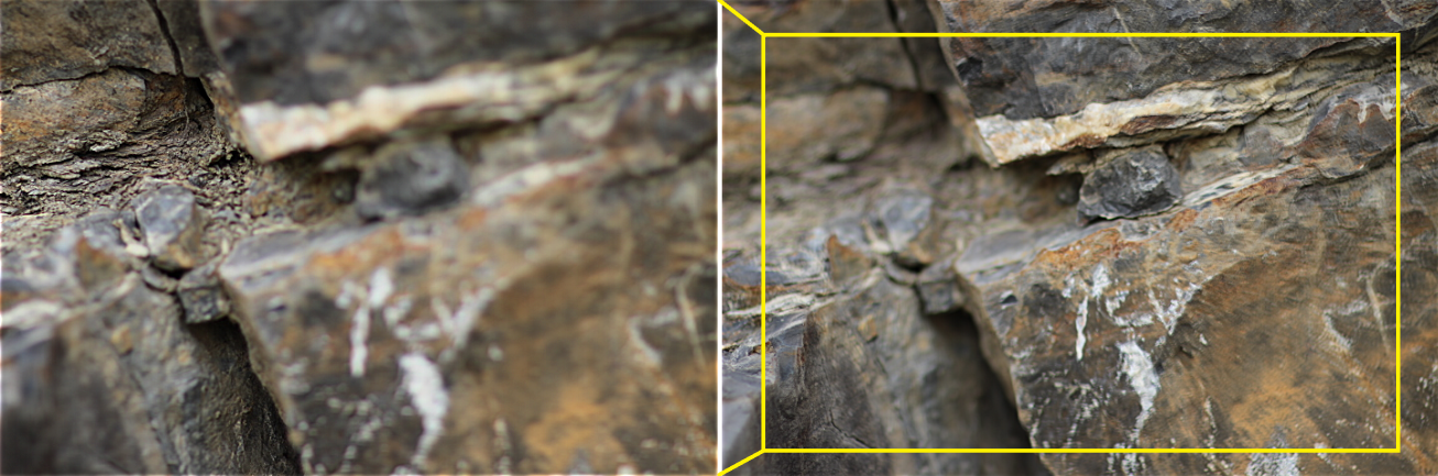
Figure 1. Different scaling and different sharp and non-sharp regions in images acquired by the classic camera positioned at different distances from the 3D relief - the first (a) and the fourth (b) image of a series of eight images, limestone, locality Brno - Hady, Czech Republic.

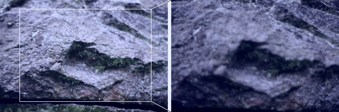
Figure 2. Different scaling and different sharp and non-sharp regions in images acquired by the classic camera positioned at different distances from the 3D relief of the first (a) and the sixteenth (b) image of a series of sixteen images, blue marble, locality Nedvedice, Czech Republic.

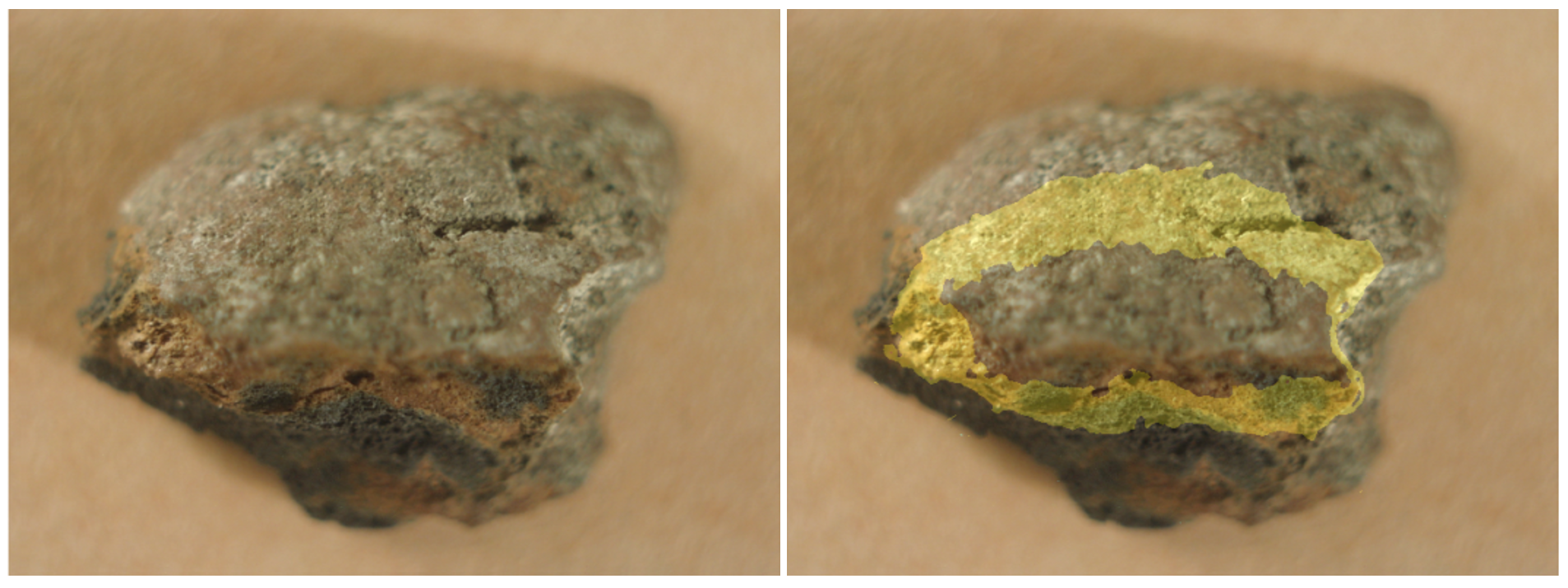
Figure 3. One of seven optical cuts of a lava fragment. Locality Vesuvio, Italy

6.2. Image Registration

Figure 4 shows the photos of Figure 2 but this time displayed in supplementary pseudo-colours. If these images were totally identical, then the arithmetic mean of the blue-green image on the left and orange image on the right would be „perfectly gray“. The arithmetic mean of these images is shown in Figure 5 on the left. Clearly, the components of this mean value are very different – the values of the orange image are bigger in the yellow parts of the mean vale while the values of the blue-green image are bigger in the blue-violet parts of the mean value. In Fig. 5 onthe right, the same construction was used after the registration. The very low colour saturation of the arithmetic mean (of the images) testifies to a very good conformity. Of course, the arithmetic mean cannot be a „perfect gray“ in this particular case because the original images also differ in the sharp parts.

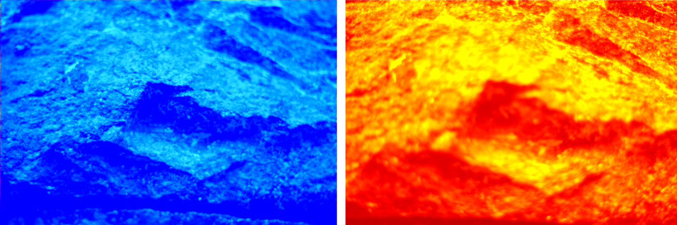
Figure 4. The first (a) and the fifteenth (b) image of a series of fifteen images of blue marble (see Fig. 3) displayed in supplementary pseudo-colours. 

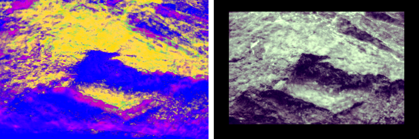
Figure 5. The arithmetic mean of the images of Figure 4 before registration (on the left), after registration (on the right).

6.3. 2D and 3D Reconstructions

We can see optical cuts detected in the data of Figure 2 in Figure 6. 2D reconstruction (sharp 2D Image) of the same data using the same criterion in Figure 7. Echelon approximation is a simple method for constructing a rough 3D model of the object, where all points belonging to the same optical cut have the same height – the height of the corresponding zone of sharpness - see Figure 8.

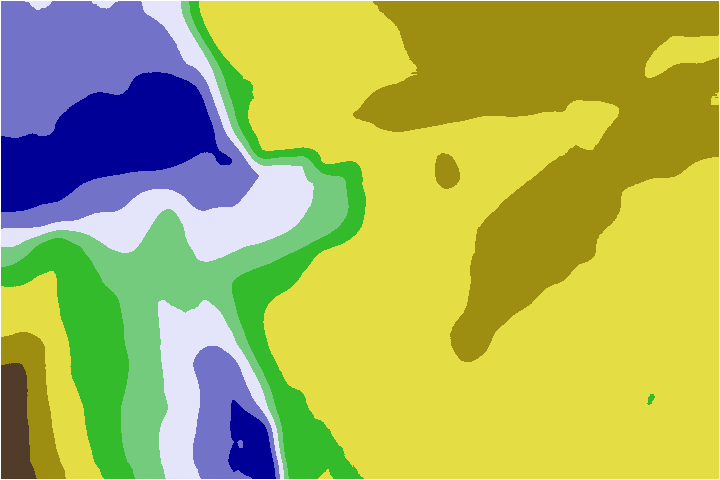
Figure 6. Optical cuts detected in multifocal Image from Figure 1.

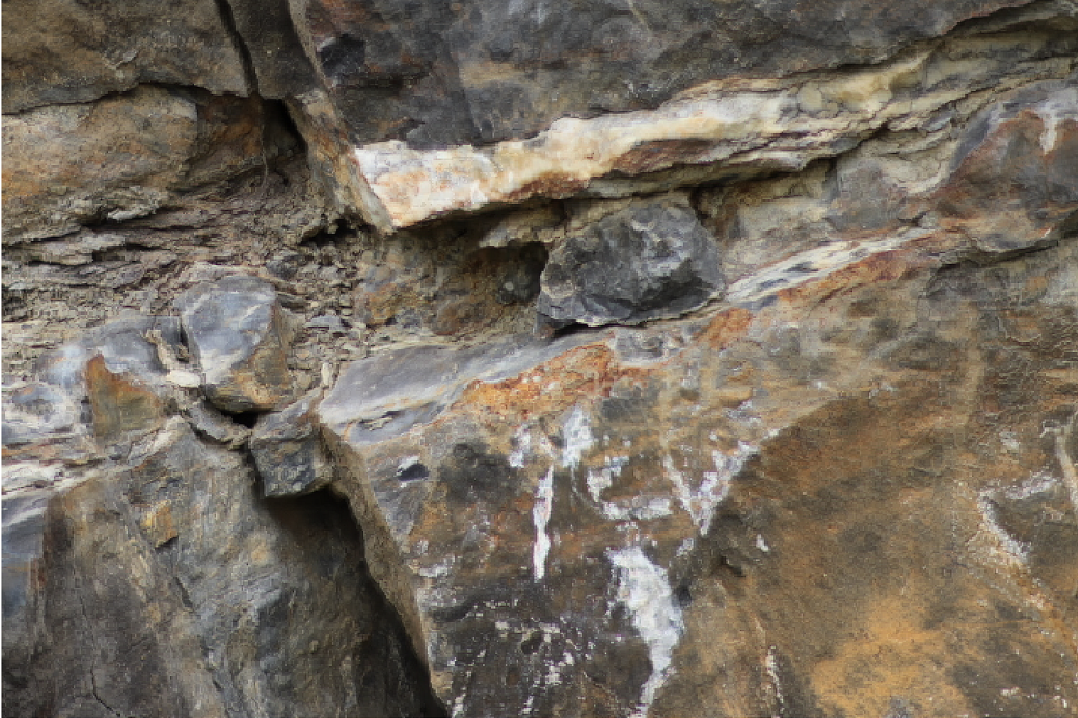
Figure 7. 2D reconstruction (sharp image) of data from Figure 1.

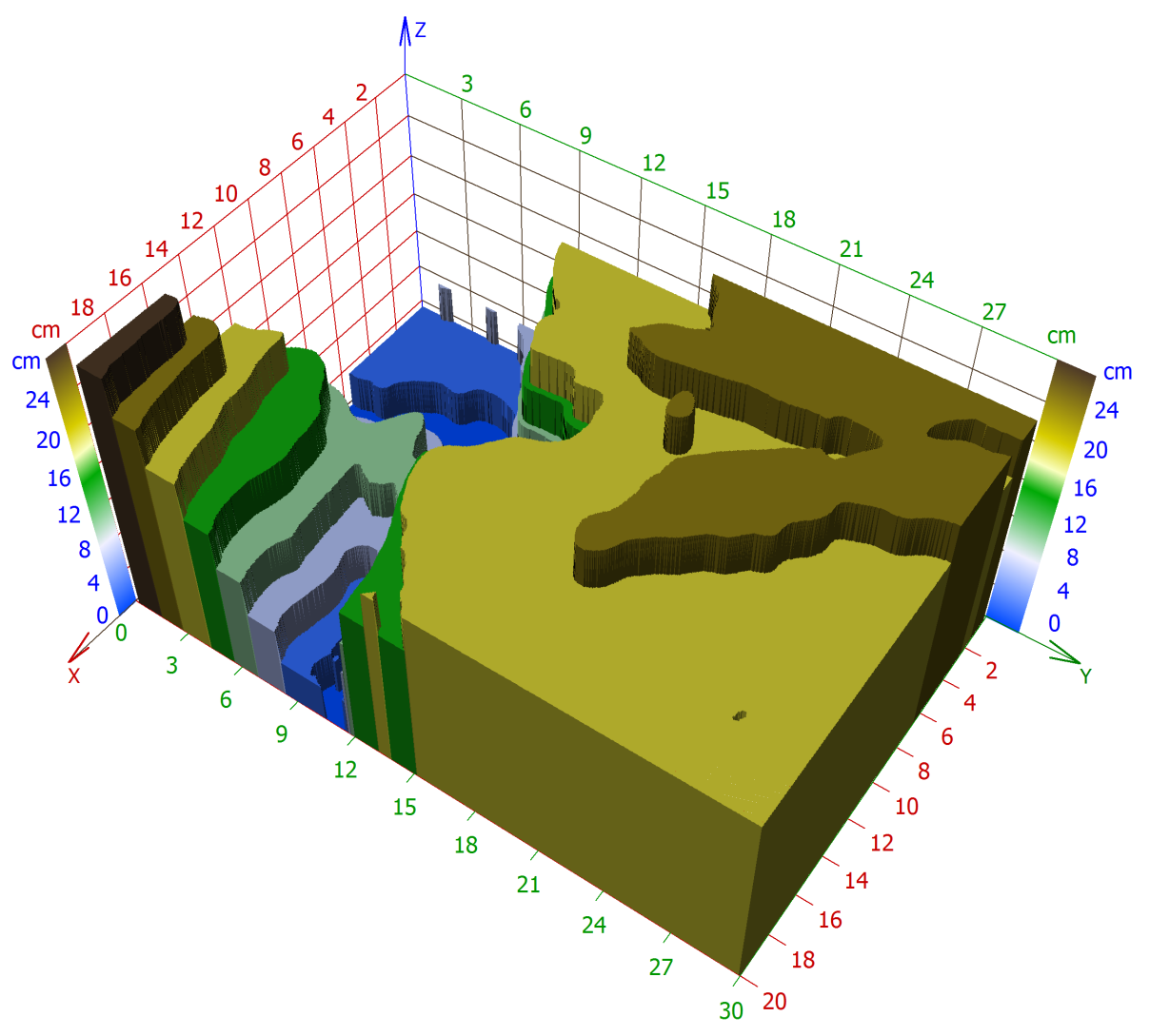
Figure 8. A 3D echelon approximation of the limestone sample by the optical cuts used in Figure 1.

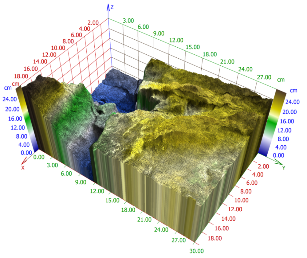
Figure 9. A 3D reconstruction of the limestone sample from Figure 1.