Deep Learning Architectures for Multivariate Time-Series Forecasting

Version	Summary	Created by	Modification	Content Size	Created at	Operation
1		Vasilis Papastefanopoulos	--	3129	2023-10-27 09:19:04	\|
2	layout	Camila Xu	Meta information modification	3129	2023-10-27 09:51:20	\|

This entry is adapted from the peer-reviewed paper 10.3390/smartcities6050114

Deep learning algorithms, renowned for their ability to extract intricate patterns from complex datasets, have proven particularly adept at handling the multifaceted time-series data characteristic of smart city IoT applications. Deep learning architectures model complex relationships through a series of nonlinear layers—the set of nodes of each intermediate layer capturing the corresponding feature representation of the input.

machine learning deep learning IoT smart cities time series

1. Introduction

A smart city is a place where traditional networks and services are improved by utilizing and embracing contemporary technological principles for the benefit of its citizens ^[1]. Smart cities are being rapidly implemented to accommodate the continuously expanding population in urban cities and provide them with increased living standards ^[2]. Going beyond the use of digital technologies for better resource use and less emissions, the development of smart cities entails smarter urban transportation networks, more responsive and interactive administration, improved water supply and waste disposal facilities, more efficient building lighting and heating systems, safer public places, and more. To this end, smart cities employ Internet of Things (IoT) devices, such as connected sensors, embedded systems, and smart meters, to collect various measurements at regular intervals (time-series data), which are subsequently analyzed and ultimately used to improve infrastructure and services ^[3].

Deep learning algorithms ^[4], renowned for their ability to extract intricate patterns from complex datasets, have proven particularly adept at handling the multifaceted time-series data characteristic of smart city IoT applications. These algorithms are designed to capture the dynamics of multiple time series concurrently and harness interdependencies among these series, resulting in more robust predictions ^[5]. Consequently, deep learning techniques have found application in various time-series forecasting scenarios across diverse domains, such as retail ^[6], healthcare ^[7], biology ^[8], medicine ^[9], aviation ^[10], energy ^[11], climate ^[12], automotive industry ^[13] and finance ^[14].

Remarkable examples of these technologies in action include Singapore’s Smart Nation Program around traffic-flow forecasting, Beijing’s Environmental Protection Bureau ‘Green Horizon’, the City of Los Angeles’ ‘Predicting What We Breathe’ air-quality forecasting projects, and the United States Department of Energy SunShot initiative around renewable energy forecasting. More specifically, in Singapore, the Land Transport Authority has created a traffic management system powered by AI that analyzes real-time data to optimize traffic flow and alleviate congestion. In Beijing, IBM’s China Research Lab has developed one of the world’s most advanced air-quality forecasting systems, while across multiple cities in the United States, IBM is making renewable energy-demand and supply forecasts.

Beyond their technical implications, the implementation of such technologies brings profound socioeconomic and environmental outcomes for cities and their residents ^[15]. Indicatively, it can foster economic growth by attracting talented individuals and entrepreneurs, potentially turning cities into innovation hubs, which, in turn, can lead to job creation and increased economic competitiveness ^[16]. As smart cities become more prosperous through economic growth, healthcare and education become more accessible and more inclusive, which results in more engaged and empowered citizens, contributing to social cohesion and overall well-being ^[17]. Moreover, AI-driven efficiency improvements in resource management can make cities more environmentally sustainable, addressing global challenges such as climate change ^[18].

There have been several surveys around deep learning for time-series forecasting, both in theoretical ^[5] and experimental ^[19] contexts. Looking at smart cities, deep learning has been used in various domains, but since this is still an emerging application area, only a few surveys have studied the current state-of-the-art models. Many of these, such as ^[20]^[21], describe deep learning as part of a broader view of machine learning approaches and examine a limited number of models. Other studies focusing on deep learning methods consider a wide set of data types, such as text and/or images ^[22]^[23]^[24]^[25], or address tasks beyond forecasting (e.g., classification), thus not providing a comprehensive overview on time-series forecasting in IoT-based smart city applications.

2. Deep Learning Architectures for Multivariate Time-Series Forecasting

Deep learning architectures model complex relationships through a series of nonlinear layers—the set of nodes of each intermediate layer capturing the corresponding feature representation of the input ^[26]. In a time-series context, these feature representations correspond to relevant temporal information up to that point in time, encoded into some latent variable at each step. In the final layer, the very last encoding is used to make a forecast. In this section, the most common types of deep learning building blocks for multivariate time-series forecasting are outlined.

2.1. Recurrent Neural Networks

Recurrent neural networks have a long and well-established history when it comes to time-series forecasting ^[27] that continues to date. The core building block of RNNs is the RNN cells that essentially act as an internal memory state. Their purpose is to maintain a condensed summary of past information deemed useful by the network for forecasting future values. At each time step, the network is presented with fresh observations, and cells are updated accordingly with new information. The standard structure of an RNN and its unfolded-in-time version are shown in Figure 1. In the case of multivariate time series, the inputs x and outputs t are multidimensional in each of the time steps.

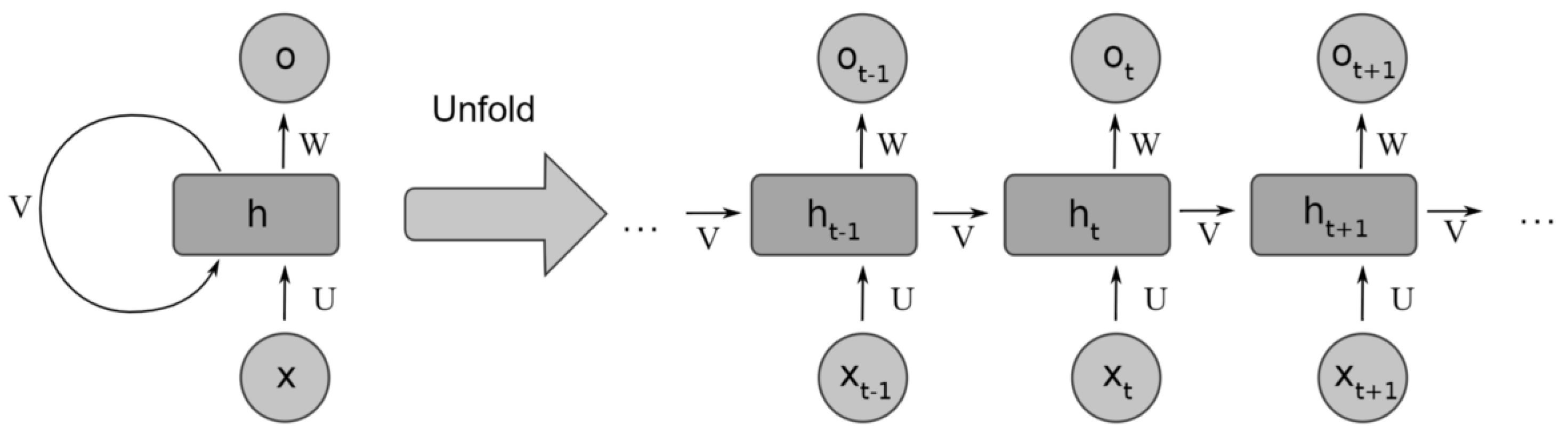
Figure 1. RNN unfolding—adapted from ^[28].

Older versions of RNNs were notorious for failing to adequately capture long-term dependencies, a problem commonly known as ’exploding and vanishing gradients’ ^[29]. More specifically, the lack of restriction on their look-back window range meant that the RNNs cells were unable to contain all the relevant information from the beginning of the sequence ^[30]. The advent of long short-term memory networks (LSTMs) ^[31] and other closely related variants, such as the gated recurrent units (GRUs ^[32]), largely alleviated this problem, by allowing the gradients to flow more stably within the network. In Figure 2, the different cells used by the LSTMs and GRUs are displayed.

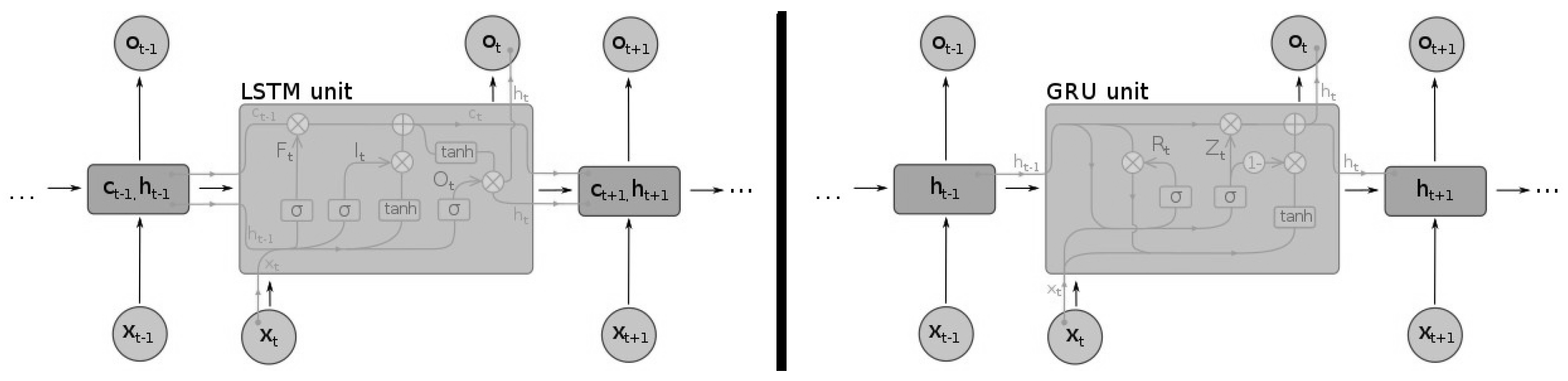
Figure 2. Different recurrent neural network cells: LSTM (left) and GRU (right)—adapted from ^[33].

Another shortcoming of conventional RNNs was the inability to make use of future time steps. To overcome this limitation, a new type of architecture, bidirectional RNNs (BiRNNs), was proposed by Schuster and Paliwal ^[34]. The novelty of BiRNNs was that they could be trained in both time directions at the same time, using separate hidden layers for each direction: forward layers and backward layers. Later on, Graves and Schmidhuber ^[35] introduced the LSTM cell to the BiRNN architecture, creating an improved version: the bidirectional LSTM (BiLSTM). Using the same principles, the bidirectional paradigm can be extended to GRUs to create BiGRU networks. A very common and powerful end-to-end approach to sequence modeling that utilizes LSTMs, GRUs, or their bidirectional versions is the sequence-to-sequence (Seq2seq) or encoder-decoder framework ^[36]. This framework originally had a lot of success in natural language processing tasks, such as machine translation, but can also be used in time-series prediction ^[37]. Under this framework, a neural network (the encoder) is used to encode the input data in a fixed-size vector, while another neural network takes the produced fixed-size vector as its own input to produce the target time series. Any of the mentioned RNN variants can act as the encoder or the decoder. Such an architecture can produce an entire target sequence all at once. All these advances and improvements to RNNs have resulted in them being established as the driving force behind many modern state-of-the-art multivariate time-series forecasting architectures, which use them as their main building blocks ^[38]^[39]^[40]^[41]^[42].

When utilizing RNNs and their variants, careful attention should be given to their hyperparameter tuning ^[43], especially in the selection of the number of hidden units, hidden layers, the learning rate, and the batch size. The number of hidden units and layers should align with the data complexity, and the more complex the data, the higher the number of layers and neural networks as a general rule of thumb. Adaptive learning rate techniques are essential to address nonstationarity, while the right batch size can ensure a smoother learning process. Lastly, for such models to thrive, it is important that the length of the input sequences should match the time patterns in it, especially if long-term connections are to be captured.

2.2. Convolutional Neural Networks

Convolutional neural networks were originally used for computer vision tasks. By making strong, but to a great degree correct, assumptions about the nature of images in terms of the stationarity of statistics and locality of pixel dependencies, CNNs are able to learn meaningful relationships and extract powerful representations ^[44].

CNNs typically consist of a series of convolutional layers followed by pooling layers, with one or more dense layers in the end. Convolutional layers perform a convolution operation of their input series with a filter matrix to construct high-level representations. The purpose of the pooling operation is to reduce the dimensionality of these representations while preserving as much information as possible. In addition, the produced representations are rotationally and positionally invariant. CNNs for time-series data, usually referred to as temporal CNNs and similar to standard/spatial CNNs, make invariance assumptions. In this case, however, such assumptions are about time instead of space, as they maintain the same set of filter weights across each time step. For CNNs to be transferred from the domain of computer vision to time-series forecasting, some modifications are needed ^[45]^[46]. A main concern is that the look-back window of CNNs is controlled by and limited by the size of its filter, also known as the receptive field. As a result, choosing the right filter size is crucial for the network’s capability to pick up all the relevant historical information, and finding an optimal size is not an easy task and is usually considered part of the hyperparameter tuning process ^[46]. Another consideration is related to the leakage of data from the future into the past; in ^[45], the so-called causal convolutions were developed to make sure that there is no leakage from the future into the past and only past information is used for forecasting. Lastly, to capture long-term temporal dependencies, a combination of very deep networks, augmented with residual layers, along with dilated convolutions, are employed, which are able to maintain very long effective history sizes ^[46]. An example of a CNN architecture for multivariate time-series forecasting can be seen in Figure 3. Since the number of parameters grows in line with the size of the look-back window, the use of standard convolutional layers can be computationally expensive, especially in cases where strong long-term dependencies are formed. To decrease the computational burden but maintain the desired results, newer architectures ^[45]^[47] often employ so-called dilated convolutional layers. Dilated convolutions can be viewed as convolutions of a downsampled version of the lower-level features, making it much less expensive to incorporate information from past time steps. The degree of downsampling is controlled by the dilation rate, applied on a layer basis. Dilated convolutions can, therefore, gradually accumulate information from various time blocks by increasing the dilation rate with each layer, allowing for more efficient utilization of historic information ^[5].

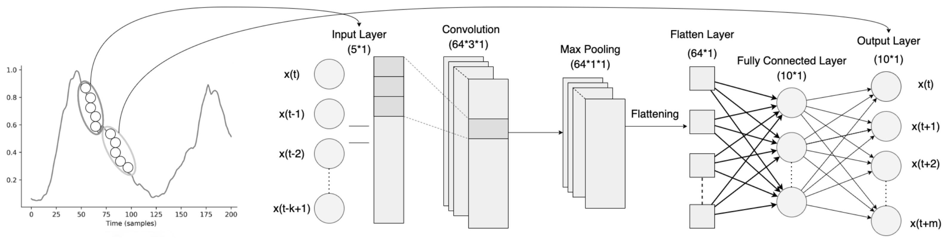
Figure 3. Convolutional neural network architecture for multivariate time-series forecasting—adapted from ^[48].

When it comes to hyperparameter tuning, focus should be directed towards the alignment of the number of filters, the filter sizes, the number of convolutional layers, and pooling strategies with the inherent patterns of the data ^[47]. More specifically, the more intricate and diverse the data are, the greater the number of filters and layers needed to capture it. Longer sequences contain more information and context and usually require larger filters to capture broader patterns and dependencies over extended periods. If the data are noisy, then pooling layers can help cut through the noise and improve the model’s focus on the features that matter.

2.3. Attention Mechanism

LSTMs acted to mitigate the problem of vanishing gradients, however, they did not eradicate it. While, in theory, the LSTM memory can hold and preserve information from the previous state, in practice, due to vanishing gradients, the information retained by these networks at the end of a long sequence is deprived of any precise, contextual, or extractable information about preceding states.

This problem was addressed by the attention mechanism ^[49]^[50], originally used in transformer architectures for machine translation ^[51]^[52]^[53]. Attention is a technique that helps neural networks focus on the more important parts of the input data and deprioritize the less important ones. Which parts are more relevant is learned by the network through the input data itself and is derived by the context. This is achieved by making all the previous states at any preceding point along the sequence available to the network; through this mechanism the network can access all previous states and weight them according to a learned measure of relevancy, providing relevant information even from the distant past. Outside of natural language processing tasks, attention-based architectures have demonstrated state-of-the-art performance in time-series forecasting ^[54]^[55]^[56]. The two most broadly used attention techniques are dot-product attention and multihead attention. The former calculates attention as the dot product between vectors, while the latter incorporates various attention mechanisms—usually different attention outputs are independently computed and are subsequently concatenated and linearly transformed into the expected dimension. These two different types of attention are shown in Figure 4.

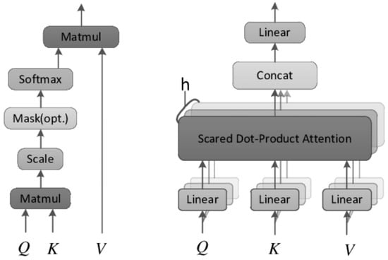
Figure 4. Attention mechanisms: dot-product (left) vs. multihead (right)—adapted from ^[57].

The choice of hyperparameters in attention models for time-series forecasting can be heavily influenced by the specific characteristics of the time-series data ^[58]. For instance, the series length can affect the number of attention heads and the attention window size. Longer sequences may require more attention heads to capture various dependencies and a wider attention window to consider longer-term patterns. Seasonality in the data may necessitate specialized attention mechanisms or attention spans to focus on recurring patterns, while nonstationary data may benefit from adaptive attention mechanisms to adapt to changing dynamics. The choice of attention mechanism type may also depend on the data characteristics; self-attention mechanisms like those in transformers are known for their ability to capture complex dependencies and intricate patterns.

2.4. Graph Neural Networks

In some cases, time-series problems are challenging because of the complex temporal and spatial dependencies. RNNs and temporal CNNs are capable of modeling the former, but they cannot solve the latter. Normal CNNs, to some degree, alleviate the problem by modeling the local spatial information; however, they are limited to cases of Euclidean structure data. Graph neural networks (GNNs), designed to exploit the properties of non-Euclidean structures, are capable of capturing the underlying spatial dependencies, offering a new perspective on approaching such forecasting problems, e.g., traffic-flow forecasting ^[59].

GNN-based approaches are generally divided into two categories: spectral and nonspectral approaches. For spectral approaches to function, a well-defined graph structure is required ^[60]. Therefore, a GNN trained on a specific structure that defines the relationships among the different variables cannot be directly applied to a graph with a different structure. On the other hand, nonspectral approaches define convolutions directly on the graph, operating on groups of spatially close neighbors; this technique operates by sampling a fixed-size neighborhood of each node, and then performing some aggregation function over it ^[61]. In any case, variables from multivariate time series can then be considered as nodes in a graph, where the state of a node depends on the states of its neighbors, forming latent spatial relationships.

To capture the spatial dependencies among their nodes, GNNs use a different type of convolution operation, called graph convolution ^[60]. The basic idea of graph convolutions is similar to that of traditional convolutions, often used in images, where a filter is applied to a local region of an image and produces a new value for each pixel in that region. Similarly, graph convolutions apply a filter to a local neighborhood of nodes in the graph, and a new value is computed for each node based on the attributes of its neighbors. This way, node representation is updated by aggregating information from their neighbors. Graph convolutions are typically implemented using some message-passing scheme that propagates information through the graph ^[62]. In Figure 5, such convolution operations on different nodes of a graph are exemplified.

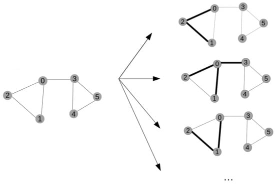
Figure 5. Graph convolutions applied to different nodes of a graph. Each node is denoted by a number (0–5).

Regarding the temporal dependencies, some GNN-based architectures may still use some type of RNN or temporal CNN to learn the temporal dependencies ^[63]^[64], while others have tried to jointly model both the intraseries temporal patterns and interseries correlations ^[65]. A new type of GNN, which incorporates the attention mechanism, called a graph attention network (GAT), was introduced by Veličković et al. ^[61]. The idea is to represent each node in the graph as a weighted average of the nonlinearly transformed features of only the neighboring nodes, using the attention coefficients. As a result, different importances are assigned to different nodes within a neighborhood, and at the same time, the need to know the entire graph structure upfront is eliminated. Even though recent advances in GNNs have demonstrated great potential by achieving state-of-the-art performance in various tasks, they have not been applied to time-series forecasting tasks to such a large extent as their RNN or CNN counterparts ^[66].

When applying GNNs to time-series data structured as graphs, key considerations captured by hyperparameters include defining node and edge representations, determining the number of message-passing layers to handle temporal dependencies, choosing aggregation functions for gathering information from neighboring nodes, and addressing dynamic graph structures for evolving time series ^[67]. More specifically, while simpler GNN architectures with fewer layers can suffice for short sequences or stable trends, longer sequences often require deeper GNNs to capture extended dependencies. Highly variable data patterns may demand more complex GNN structures, while the presence of strong seasonality may warrant specialized aggregation functions. Finally, the graph structure should mirror the relationships between variables in the time series, e.g., directed, weighted, or otherwise, to enable effective information propagation across the network.

2.5. Hybrid Approaches

Hybrid approaches combine different deep learning architectures, bringing together the benefits of each. Generally speaking, architectures integrating more than one learning algorithm have been shown to produce methods of increased robustness and predictive power, compared to single-model architectures ^[68]. Their increased robustness stems from the fact that, by using multiple types of neural networks, hybrids are less prone to noise and missing data, which helps them learn more generalizable representations of the data. At the same time, the combination of different types of neural networks increases the flexibility of the model, allowing it to be more easily tailored to the specific characteristics and patterns of the given time-series data ^[69]. A common approach in deep learning hybrids for time-series forecasting has been to combine models that are good at feature extraction such as CNNs or autoencoders, with models capable of learning temporal dependencies among those features, such as LSTMS, GRUs, or BiLSTMs. In Figure 6, a commonly used CNN–LSTM hybrid architecture is depicted.

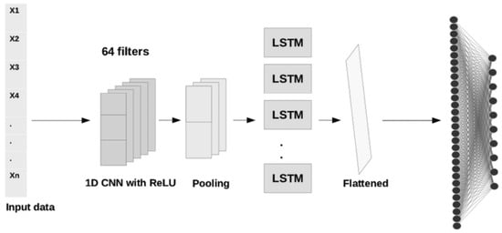
Figure 6. A simple CNN–LSTM hybrid architecture—adapted from ^[70].

Despite their advantages, hybrid models are often more computationally intensive, leading to longer training times and demanding more resources. Additionally, hyperparameter tuning becomes more challenging due to the increased complexity and the need to optimize settings for multiple components. They should, therefore, be considered mostly in cases where simpler models do not perform adequately.

References

Pribyl, O.; Svitek, M.; Rothkrantz, L. Intelligent Mobility in Smart Cities. Appl. Sci. 2022, 12, 3340.
Silva, B.N.; Khan, M.; Han, K. Towards sustainable smart cities: A review of trends, architectures, components, and open challenges in smart cities. Sustain. Cities Soc. 2018, 38, 697–713.
Panagiotakopoulos, T.; Kiouvrekis, Y.; Mitshos, L.M.; Kappas, C. RF-EMF exposure assessments in Greek schools to support ubiquitous IoT-based monitoring in smart cities. IEEE Access 2023, 190, 7145–7156.
LeCun, Y.; Bengio, Y.; Hinton, G. Deep learning. Nature 2015, 521, 436–444.
Lim, B.; Zohren, S. Time-series forecasting with deep learning: A survey. Philos. Trans. R. Soc. A 2021, 379, 20200209.
Böse, J.H.; Flunkert, V.; Gasthaus, J.; Januschowski, T.; Lange, D.; Salinas, D.; Schelter, S.; Seeger, M.; Wang, Y. Probabilistic demand forecasting at scale. Proc. VLDB Endow. 2017, 10, 1694–1705.
Kaushik, S.; Choudhury, A.; Sheron, P.K.; Dasgupta, N.; Natarajan, S.; Pickett, L.A.; Dutt, V. AI in healthcare: Time-series forecasting using statistical, neural, and ensemble architectures. Front. Big Data 2020, 3, 4.
Leise, T.L. Analysis of nonstationary time series for biological rhythms research. J. Biol. Rhythm. 2017, 32, 187–194.
Lynn, L.A. Artificial intelligence systems for complex decision-making in acute care medicine: A review. Patient Saf. Surg. 2019, 13, 1–8.
Vonitsanos, G.; Panagiotakopoulos, T.; Kanavos, A.; Tsakalidis, A. Forecasting air flight delays and enabling smart airport services in apache spark. In Proceedings of the In Artificial Intelligence Applications and Innovations, AIAI 2021 IFIP WG 12.5 International Workshops, Crete, Greece, 25–27 June 2021; pp. 407–417.
Martínez-Álvarez, F.; Troncoso, A.; Asencio-Cortés, G.; Riquelme, J.C. A survey on data mining techniques applied to electricity-related time series forecasting. Energies 2015, 8, 13162–13193.
Mudelsee, M. Trend analysis of climate time series: A review of methods. Earth-Sci. Rev. 2019, 190, 310–322.
Nousias, S.; Pikoulis, E.V.; Mavrokefalidis, C.; Lalos, A. Accelerating deep neural networks for efficient scene understanding in multi-modal automotive applications. IEEE Access 2023, 11, 28208–28221.
Sezer, O.B.; Gudelek, M.U.; Ozbayoglu, A.M. Financial time series forecasting with deep learning: A systematic literature review: 2005–2019. Appl. Soft Comput. 2020, 11, 106181.
Akindipe, D.; Olawale, O.W.; Bujko, R. Techno-economic and social aspects of smart street lighting for small cities—A case study. Sustain. Cities Soc. 2022, 84, 103989.
Appio, F.P.; Lima, M.; Paroutis, S. Understanding Smart Cities: Innovation ecosystems, technological advancements, and societal challenges. Technol. Forecast. Soc. Chang. 2019, 142, 1–14.
Neirotti, P.; De Marco, A.; Cagliano, A.C.; Mangano, G.; Scorrano, F. Current trends in Smart City initiatives: Some stylised facts. Cities 2014, 38, 25–36.
Trindade, E.P.; Hinnig, M.P.F.; da Costa, E.M.; Marques, J.S.; Bastos, R.C.; Yigitcanlar, T. Sustainable development of smart cities: A systematic review of the literature. J. Open Innov. Technol. Mark. Complex. 2017, 3, 1–14.
Lara-Benítez, P.; Carranza-García, M.; Riquelme, J.C. An experimental review on deep learning architectures for time series forecasting. Int. J. Neural Syst. 2021, 31, 2130001.
Gharaibeh, A.; Salahuddin, M.; Hussini, S.; Khreishah, A.; Khalil, I.; Guizani, M.; Al-Fuqaha, A. Smart cities: A survey on data management, security, and enabling technologies. IEEE Commun. Surv. Tutor. 2017, 19, 2456–2501.
Mohammadi, M.; Al-Fuqaha, A. Enabling cognitive smart cities using big data and machine learning: Approaches and challenges. IEEE Commun. Mag. 2018, 56, 94–101.
Atitallah, S.B.; Driss, M.; Boulila, W.; Ghézala, H.B. Leveraging Deep Learning and IoT big data analytics to support the smart cities development: Review and future directions. Comput. Sci. Rev. 2020, 38, 100303.
Ciaburro, G. Time series data analysis using deep learning methods for smart cities monitoring. In Big Data Intelligence for Smart Applications; Springer: Berlin/Heidelberg, Germany, 2022; pp. 93–116.
Chen, Q.; Wang, W.; Wu, F.; De, S.; Wang, R.; Zhang, B.; Huang, X. A survey on an emerging area: Deep learning for smart city data. IEEE Trans. Emerg. Top. Comput. Intell. 2019, 3, 392–410.
Muhammad, A.N.; Aseere, A.M.; Chiroma, H.; Shah, H.; Gital, A.Y.; Hashem, I.A.T. Deep learning application in smart cities: Recent development, taxonomy, challenges and research prospects. Neural Comput. Appl. 2021, 33, 2973–3009.
Bengio, Y.; Courville, A.; Vincent, P. Representation learning: A review and new perspectives. IEEE Trans. Pattern Anal. Mach. Intell. 2013, 35, 1798–1828.
Lipton, Z.C. A Critical Review of Recurrent Neural Networks for Sequence Learning. arXiv 2015, arXiv:1506.00019.
Zhang, T.; Aftab, W.; Mihaylova, L.; Langran-Wheeler, C.; Rigby, S.; Fletcher, D.; Maddock, S.; Bosworth, G. Recent advances in video analytics for rail network surveillance for security, trespass and suicide prevention—A survey. Sensors 2022, 22, 4324.
Pascanu, R.; Mikolov, T.; Bengio, Y. On the difficulty of training recurrent neural networks. In Proceedings of the International Conference on Machine Learning. PMLR, Virtual Event, 13–18 July 2013; pp. 1310–1318.
Bengio, Y.; Simard, P.; Frasconi, P. Learning long-term dependencies with gradient descent is difficult. IEEE Trans. Neural Netw. 1994, 5, 157–166.
Hochreiter, S.; Schmidhuber, J. Long short-term memory. Neural Comput. 1997, 9, 1735–1780.
Chung, J.; Gulcehre, C.; Cho, K.; Bengio, Y. Empirical evaluation of gated recurrent neural networks on sequence modeling. In Proceedings of the NIPS 2014 Workshop on Deep Learning, Montreal, QC, Canada, 8–13 December 2014.
Han, H.; Choi, C.; Kim, J.; Morrison, R.; Jung, J.; Kim, H. Multiple-depth soil moisture estimates using artificial neural network and long short-term memory models. Water 2021, 13, 2584.
Schuster, M.; Paliwal, K.K. Bidirectional recurrent neural networks. IEEE Trans. Signal Process. 1997, 45, 2673–2681.
Graves, A.; Schmidhuber, J. Framewise phoneme classification with bidirectional LSTM and other neural network architectures. Neural Netw. 2005, 18, 602–610.
Sutskever, I.; Vinyals, O.; Le, Q.V. Sequence to sequence learning with neural networks. Adv. Neural Inf. Process. Syst. 2014, 27, 1.
Du, S.; Li, T.; Horng, S.J. Time series forecasting using sequence-to-sequence deep learning framework. In Proceedings of the 2018 9th International Symposium on Parallel Architectures, Algorithms and Programming (PAAP), Taipei, Taiwan, 26–28 December 2018; pp. 171–176.
Salinas, D.; Flunkert, V.; Gasthaus, J.; Januschowski, T. DeepAR: Probabilistic forecasting with autoregressive recurrent networks. Int. J. Forecast. 2020, 36, 1181–1191.
Rangapuram, S.S.; Seeger, M.W.; Gasthaus, J.; Stella, L.; Wang, Y.; Januschowski, T. Deep state space models for time series forecasting. Adv. Neural Inf. Process. Syst. 2018, 31, 7785–7794.
Lim, B.; Zohren, S.; Roberts, S. Recurrent Neural Filters: Learning Independent Bayesian Filtering Steps for Time Series Prediction. In Proceedings of the 2020 International Joint Conference on Neural Networks (IJCNN), Glasgow, UK, 19–24 July 2020; pp. 1–8.
Wang, Y.; Smola, A.; Maddix, D.; Gasthaus, J.; Foster, D.; Januschowski, T. Deep factors for forecasting. In Proceedings of the International Conference on Machine Learning, PMLR, Virtual Event, 13–18 July 2019; pp. 6607–6617.
Wen, R.; Torkkola, K. Deep generative quantile-copula models for probabilistic forecasting. arXiv 2019, arXiv:1907.10697.
Greff, K.; Srivastava, R.K.; Koutník, J.; Steunebrink, B.R.; Schmidhuber, J. LSTM: A search space odyssey. IEEE Trans. Neural Netw. Learn. Syst. 2016, 28, 2222–2232.
Krizhevsky, A.; Sutskever, I.; Hinton, G.E. Imagenet classification with deep convolutional neural networks. Adv. Neural Inf. Process. Syst. 2012, 25, 1097–1105.
Oord, A.v.d.; Dieleman, S.; Zen, H.; Simonyan, K.; Vinyals, O.; Graves, A.; Kalchbrenner, N.; Senior, A.; Kavukcuoglu, K. Wavenet: A generative model for raw audio. arXiv 2016, arXiv:1609.03499.
Borovykh, A.; Bohte, S.; Oosterlee, C.W. Conditional Time Series Forecasting with Convolutional Neural Networks. Statistic 2017, 1050, 16.
Bai, S.; Kolter, J.Z.; Koltun, V. An Empirical Evaluation of Generic Convolutional and Recurrent Networks for Sequence Modeling. In Universal Language Model Fine-tuning for Text Classification; Cornell University: Ithaca, NY, USA, 2018.
Chandra, R.; Goyal, S.; Gupta, R. Evaluation of deep learning models for multi-step ahead time series prediction. IEEE Access 2021, 9, 83105–83123.
Bahdanau, D.; Cho, K.; Bengio, Y. Neural machine translation by jointly learning to align and translate. arXiv 2014, arXiv:1409.0473.
Cho, K.; Van Merriënboer, B.; Gulcehre, C.; Bahdanau, D.; Bougares, F.; Schwenk, H.; Bengio, Y. Learning phrase representations using RNN encoder-decoder for statistical machine translation. arXiv 2014, arXiv:1406.1078.
Devlin, J.; Chang, M.W.; Lee, K.; Toutanova, K. Bert: Pre-training of deep bidirectional transformers for language understanding. arXiv 2018, arXiv:1810.04805.
Vaswani, A.; Shazeer, N.; Parmar, N.; Uszkoreit, J.; Jones, L.; Gomez, A.N.; Kaiser, Ł.; Polosukhin, I. Attention is all you need. In Proceedings of the Advances in Neural Information Processing Systems, Long Beach, CA, USA, 4–9 December 2017; pp. 5998–6008.
Dai, Z.; Yang, Z.; Yang, Y.; Carbonell, J.; Le, Q.V.; Salakhutdinov, R. Transformer-xl: Attentive language models beyond a fixed-length context. arXiv 2019, arXiv:1901.02860.
Fan, C.; Zhang, Y.; Pan, Y.; Li, X.; Zhang, C.; Yuan, R.; Wu, D.; Wang, W.; Pei, J.; Huang, H. Multi-horizon time series forecasting with temporal attention learning. In Proceedings of the 25th ACM SIGKDD International Conference on Knowledge Discovery & Data Mining, Anchorage, AK, USA, 4–8 August 2019; pp. 2527–2535.
Li, S.; Jin, X.; Xuan, Y.; Zhou, X.; Chen, W.; Wang, Y.X.; Yan, X. Enhancing the locality and breaking the memory bottleneck of transformer on time series forecasting. Adv. Neural Inf. Process. Syst. 2019, 32, 5243–5253.
Lim, B.; Arık, S.Ö.; Loeff, N.; Pfister, T. Temporal fusion transformers for interpretable multi-horizon time series forecasting. Int. J. Forecast. 2021, 37, 1748–1764.
Zhou, L.; Zhang, J.; Zong, C. Synchronous bidirectional neural machine translation. Trans. Assoc. Comput. Linguist. 2019, 7, 91–105.
Wen, Q.; Zhou, T.; Zhang, C.; Chen, W.; Ma, Z.; Yan, J.; Sun, L. Transformers in time series: A survey. arXiv 2022, arXiv:2202.07125.
Jiang, W.; Luo, J. Graph neural network for traffic forecasting: A survey. Expert Syst. Appl. 2022, 207, 117921.
Wu, Z.; Pan, S.; Long, G.; Jiang, J.; Chang, X.; Zhang, C. Connecting the dots: Multivariate time series forecasting with graph neural networks. In Proceedings of the 26th ACM SIGKDD International Conference on Knowledge Discovery & Data Mining, Virtual Event, 23–27 August 2020; pp. 753–763.
Veličković, P.; Cucurull, G.; Casanova, A.; Romero, A.; Liò, P.; Bengio, Y. Graph Attention Networks. In Proceedings of the International Conference on Learning Representations, Toulon, France, 24–26 April 2017.
Wu, Z.; Pan, S.; Chen, F.; Long, G.; Zhang, C.; Philip, S.Y. A comprehensive survey on graph neural networks. IEEE Trans. Neural Netw. Learn. Syst. 2020, 32, 4–24.
Yu, B.; Yin, H.; Zhu, Z. Spatio-temporal graph convolutional networks: A deep learning framework for traffic forecasting. In Proceedings of the 27th International Joint Conference on Artificial Intelligence, Stockholm, Sweden, 13–19 July 2018; pp. 3634–3640.
Li, Y.; Yu, R.; Shahabi, C.; Liu, Y. Diffusion Convolutional Recurrent Neural Network: Data-Driven Traffic Forecasting. In Proceedings of the International Conference on Learning Representations, Vancouver, BC, Canada, 30 April– 3 May 2018.
Cao, D.; Wang, Y.; Duan, J.; Zhang, C.; Zhu, X.; Huang, C.; Tong, Y.; Xu, B.; Bai, J.; Tong, J.; et al. Spectral temporal graph neural network for multivariate time-series forecasting. Adv. Neural Inf. Process. Syst. 2020, 33, 17766–17778.
Bloemheuvel, S.; van den Hoogen, J.; Jozinović, D.; Michelini, A.; Atzmueller, M. Graph neural networks for multivariate time series regression with application to seismic data. Int. J. Data Sci. Anal. 2022, 2022, 1–16.
Jin, M.; Koh, H.Y.; Wen, Q.; Zambon, D.; Alippi, C.; Webb, G.I.; King, I.; Pan, S. A survey on graph neural networks for time series: Forecasting, classification, imputation, and anomaly detection. arXiv 2023, arXiv:2307.03759.
Dietterich, T.G. Ensemble methods in machine learning. In Proceedings of the International Workshop on Multiple Classifier Systems, Cagliari, Italy, 21–23 July 2000; Springer: Berlin/Heidelberg, Germany, 2000; pp. 1–15.
Ardabili, S.; Mosavi, A.; Várkonyi-Kóczy, A.R. Advances in machine learning modeling reviewing hybrid and ensemble methods. In Proceedings of the Engineering for Sustainable Future: Selected Papers of the 18th International Conference on Global Research and Education Inter-Academia, Virtual Event, 27–29 September 2020; Springer: Berlin/Heidelberg, Germany, 2020; pp. 215–227.
Hamad, R.A.; Yang, L.; Woo, W.L.; Wei, B. Joint learning of temporal models to handle imbalanced data for human activity recognition. Appl. Sci. 2020, 10, 5293.

© Text is available under the terms and conditions of the Creative Commons Attribution (CC BY) license; additional terms may apply. By using this site, you agree to the Terms and Conditions and Privacy Policy.

Upload a video for this entry

Information

Subjects: Computer Science, Artificial Intelligence

Contributors MDPI registered users' name will be linked to their SciProfiles pages. To register with us, please refer to https://encyclopedia.pub/register :

Vasilis Papastefanopoulos

Pantelis Linardatos

Theodor Panagiotakopoulos

Sotiris Kotsiantis

View Times: 200

Update Date: 27 Oct 2023

Table of Contents

Video Upload Options

Confirm