
| Version | Summary | Created by | Modification | Content Size | Created at | Operation |
|---|---|---|---|---|---|---|
| 1 | Ngo Anh Tuan | -- | 3144 | 2023-03-14 09:39:34 | | | |
| 2 | Lindsay Dong | Meta information modification | 3144 | 2023-03-15 09:54:29 | | | | |
| 3 | Lindsay Dong | Meta information modification | 3144 | 2023-03-15 09:55:32 | | |
Video Upload Options
Quantum mechanics studies nature and its behavior at the scale of atoms and subatomic particles. By applying quantum mechanics, a lot of problems can be solved in a more convenient way thanks to its special quantum properties, such as superposition and entanglement. In the current noisy intermediate-scale quantum era, quantum mechanics finds its use in various fields of life. Following this trend, researchers seek to augment machine learning in a quantum way. The generative adversarial network (GAN), an important machine learning invention that excellently solves generative tasks, has also been extended with quantum versions. Since the first publication of a quantum GAN (QuGAN) in 2018, many QuGAN proposals have been suggested. A QuGAN may have a fully quantum or a hybrid quantum–classical architecture, which may need additional data processing in the quantum–classical interface. Similarly to classical GANs, QuGANs are trained using a loss function in the form of max likelihood, Wasserstein distance, or total variation. The gradients of the loss function can be calculated by applying the parameter-shift method or a linear combination of unitaries in order to update the parameters of the networks.
1. Introduction
1.1. Generative Adversarial Networks (GANs)
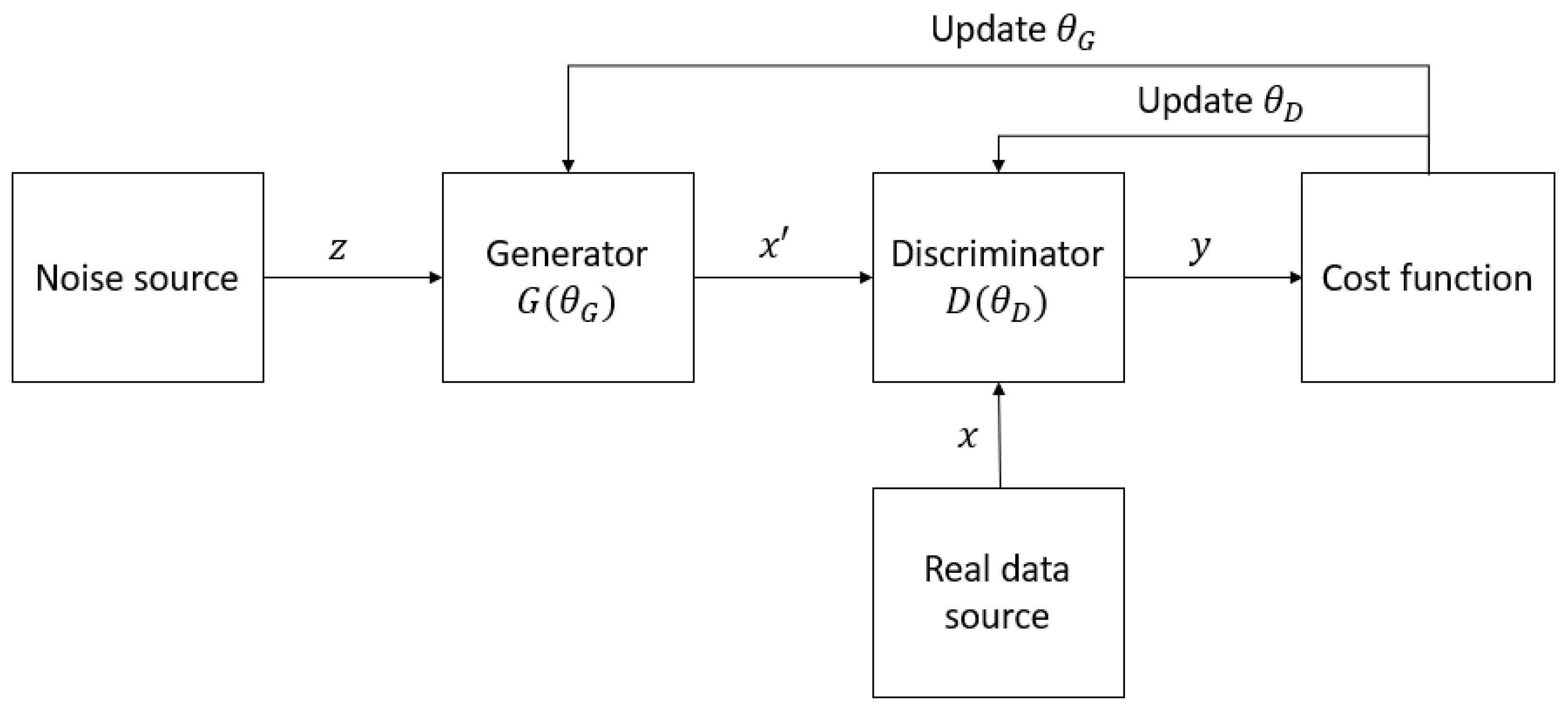
1.2. Quantum–Classical Interface
2. Structures of QuGAN
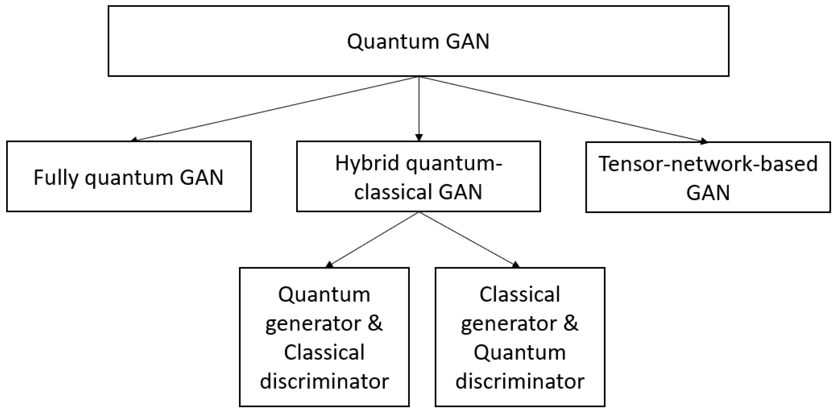
3. Optimization of QuGAN
3.1. Loss Function
3.2. Gradient Computation
3.3. Optimization and Evaluation Strategies
4. Quantum GAN Variants
4.1. Fully Quantum GANs
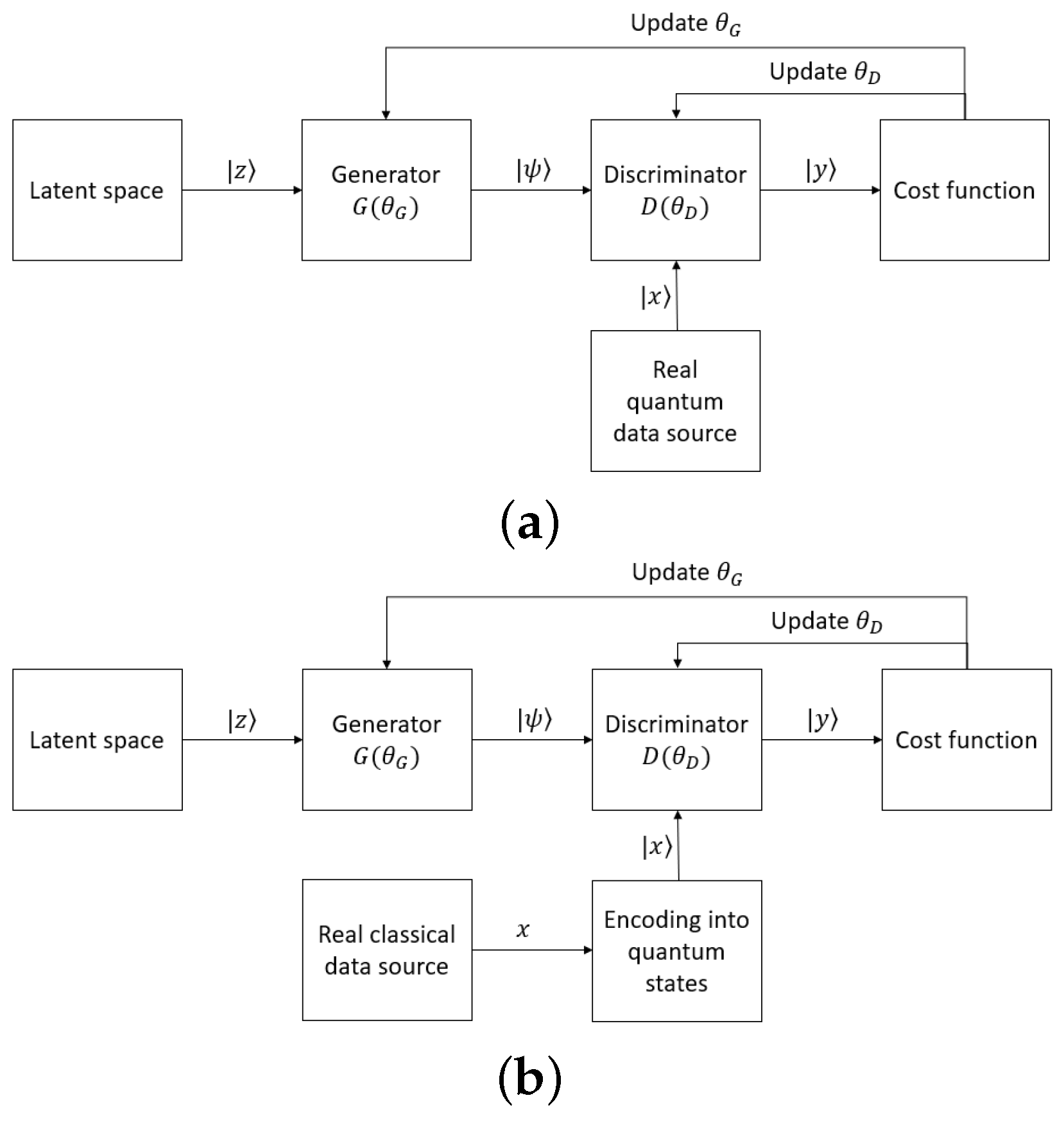
4.2. Hybrid Quantum–Classical GANs
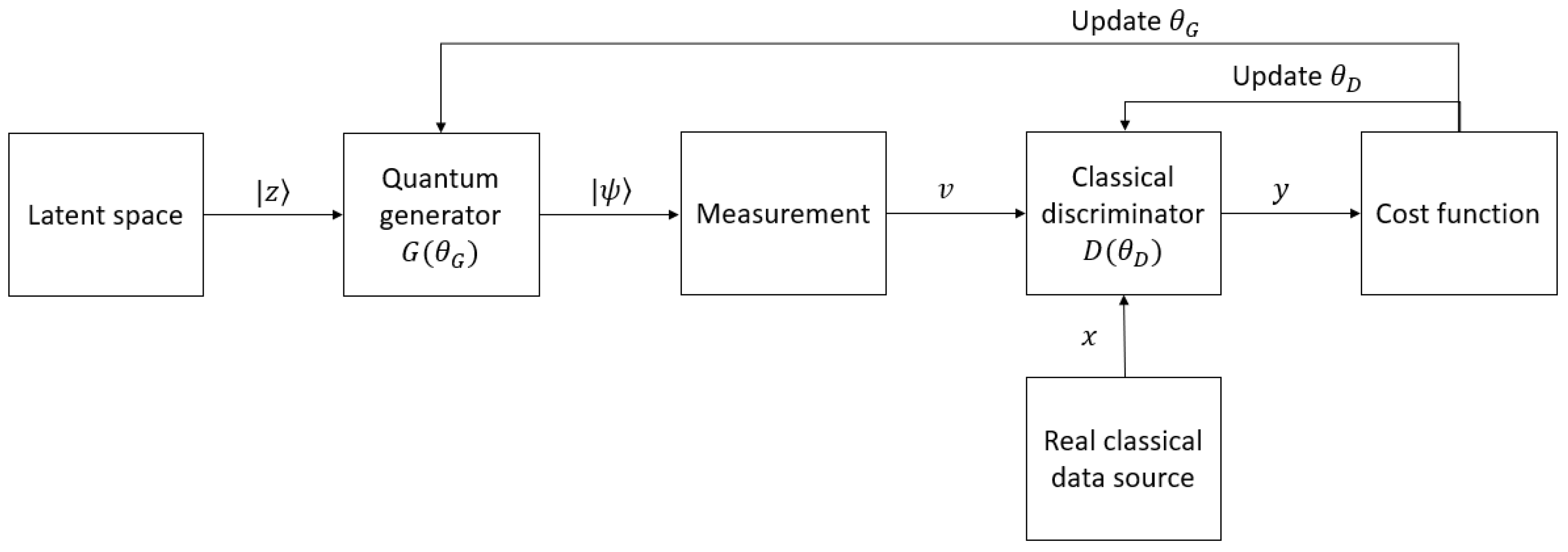
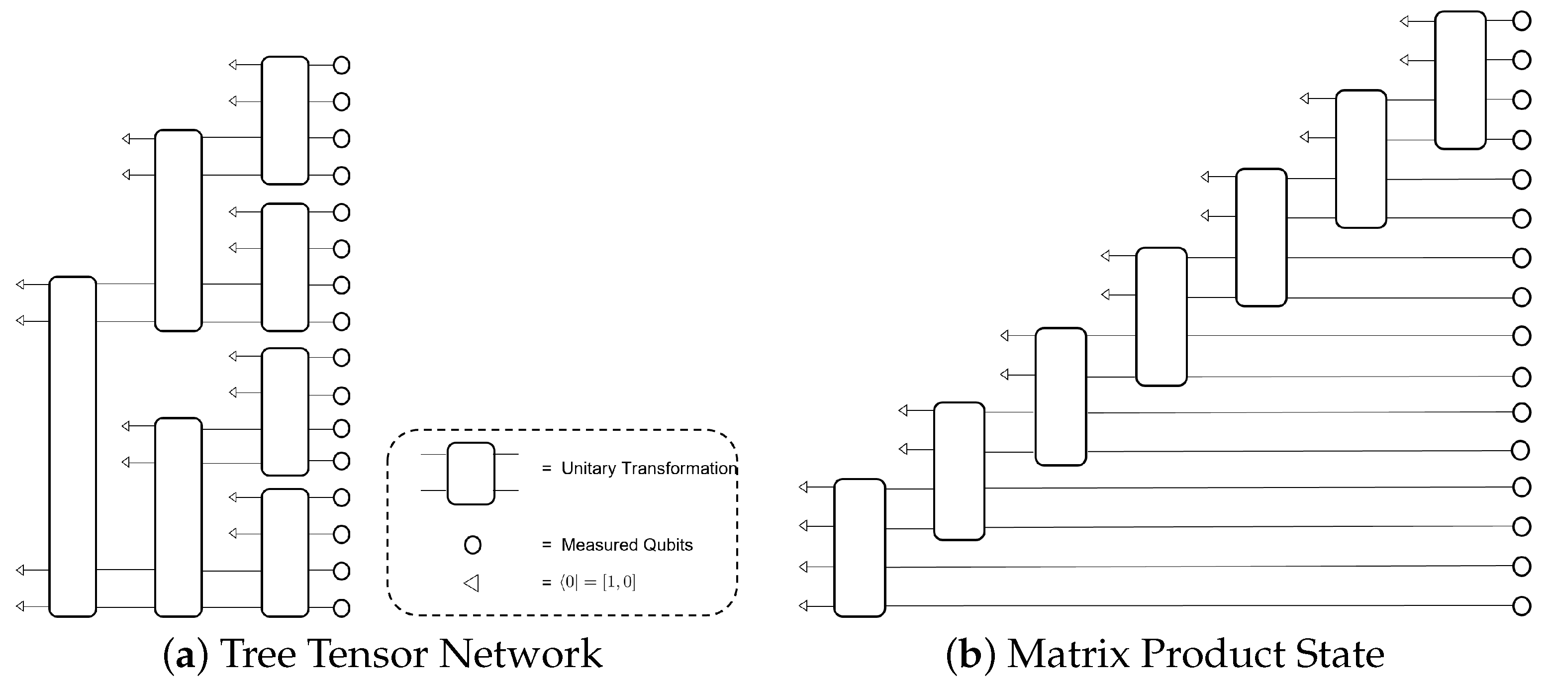
4.3. Tensor-Network-Based GANs
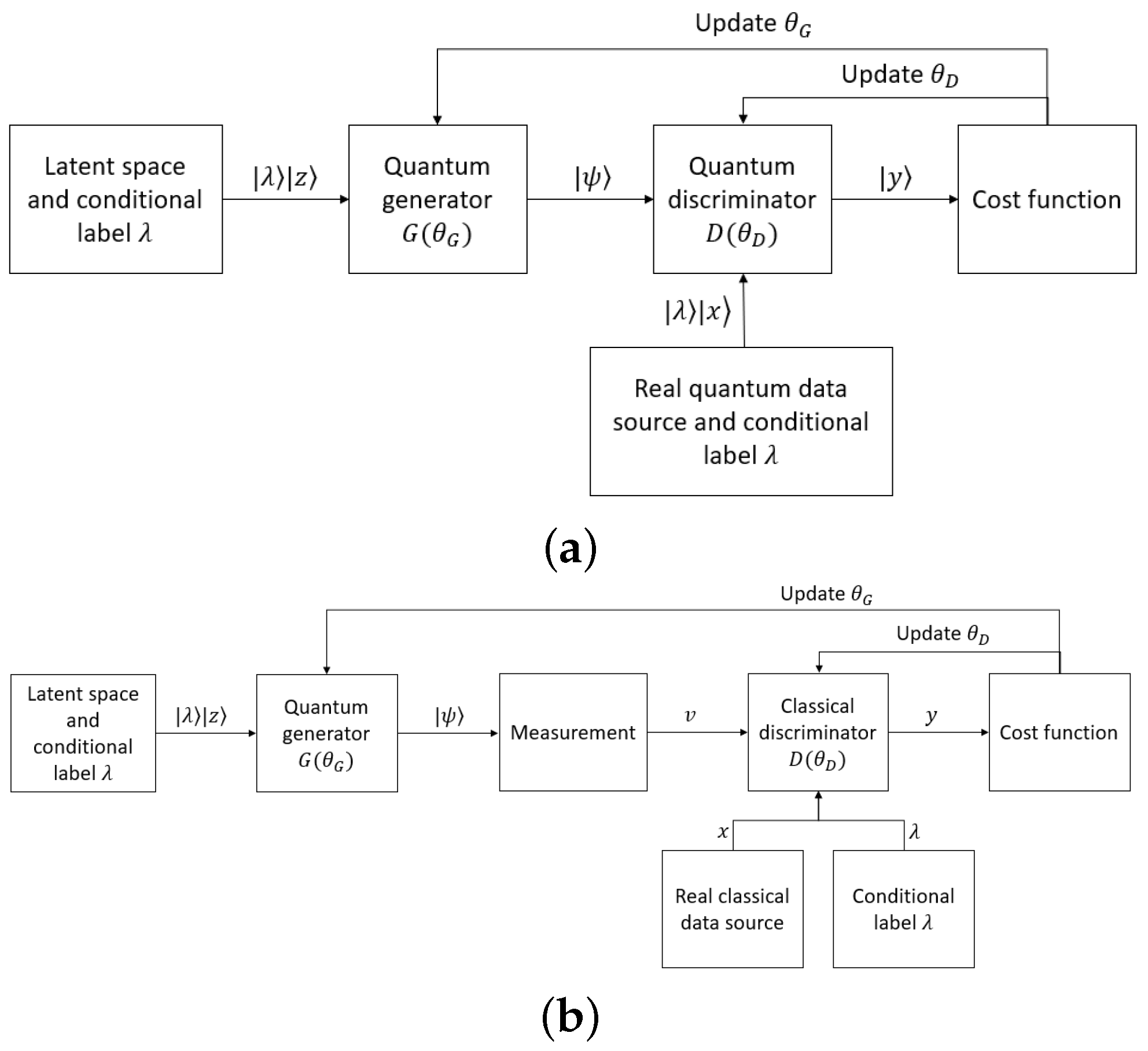
4.4. Quantum Conditional GANs
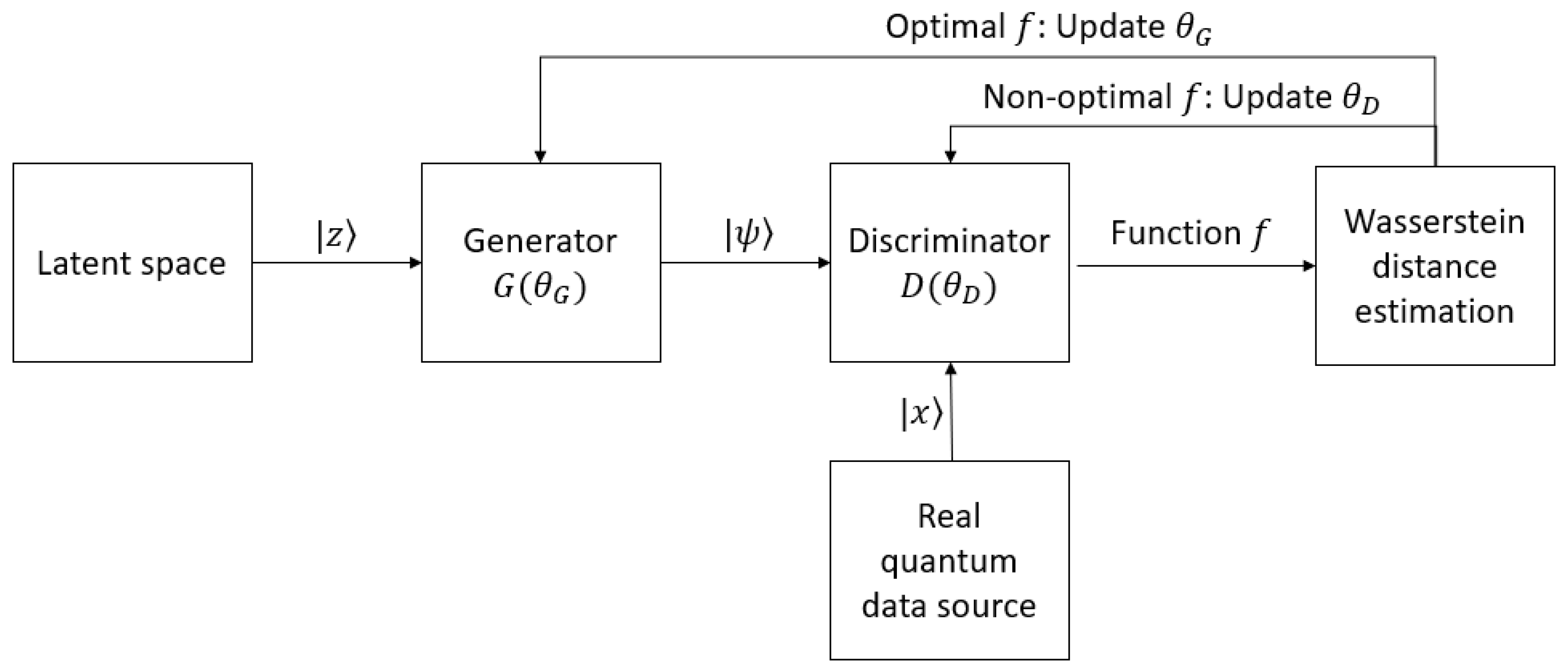
4.5. Quantum Wasserstein GANs
4.6. Quantum Patch GANs Using Multiple Sub-Generators
4.7. Quantum GANs Using Quantum Fidelity for a Cost Function
5. Conclusions
References
- Mitchell, T.; Buchanan, B.; DeJong, G.; Dietterich, T.; Rosenbloom, P.; Waibel, A. Machine Learning. Annu. Rev. Comput. Sci. 1990, 4, 417–433.
- McCulloch, W.S.; Pitts, W. A logical calculus of the ideas immanent in nervous activity. Bull. Math. Biophys. 1943, 5, 115–133.
- Rosenblatt, F. The perceptron: A probabilistic model for information storage and organization in the brain. Psychol. Rev. 1958, 65, 386–408.
- Cortes, C.; Vapnik, V. Support-vector networks. Mach. Learn. 1995, 20, 273–297.
- Hopfield, J.J. Neural networks and physical systems with emergent collective computational abilities. Proc. Natl. Acad. Sci. USA 1982, 79, 2554–2558.
- LeCun, Y.; Bengio, Y.; Hinton, G. Deep Learning. Nature 2015, 521, 436–444.
- Alam, M.M.; Mohiuddin, K.; Das, A.K.; Islam, M.K.; Kaonain, M.S.; Ali, M.H. A Reduced Feature Based Neural Network Approach to Classify the Category of Students. In Proceedings of the 2nd International Conference on Innovation in Artificial Intelligence, Shanghai, China, 9–12 March 2018; Association for Computing Machinery: New York, NY, USA, 2018; pp. 28–32.
- Luckin, R.; Holmes, W.; Griffiths, M.; Forcier, L.B. Intelligence Unleashed: An Argument for AI in Education; Pearson Education: London, UK, 2016.
- Djambic, G.; Krajcar, M.; Bele, D. Machine learning model for early detection of higher education students that need additional attention in introductory programming courses. Int. J. Digit. Technol. Econ. 2016, 1, 1–11.
- Amatya, S.; Karkee, M.; Gongal, A.; Zhang, Q.; Whiting, M.D. Detection of cherry tree branches with full foliage in planar architecture for automated sweet-cherry harvesting. Biosyst. Eng. 2016, 146, 3–15.
- Pantazi, X.E.; Moshou, D.; Bravo, C. Active learning system for weed species recognition based on hyperspectral sensing. Biosyst. Eng. 2016, 146, 193–202.
- Bouri, E.; Gkillas, K.; Gupta, R.; Pierdzioch, C. Forecasting Realized Volatility of Bitcoin: The Role of the Trade War. Comput. Econ. 2021, 57, 29–53.
- Lussange, J.; Lazarevich, I.; Bourgeois-Gironde, S.; Palminteri, S.; Gutkin, B. Modelling Stock Markets by Multi-agent Reinforcement Learning. Comput. Econ. 2021, 57, 113–147.
- Sughasiny, M.; Rajeshwari, J. Application of Machine Learning Techniques, Big Data Analytics in Health Care Sector—A Literature Survey. In Proceedings of the 2018 2nd International Conference on I-SMAC (IoT in Social, Mobile, Analytics and Cloud) (I-SMAC), Palladam, India, 30–31 August 2018; pp. 741–749.
- Hazra, A.; Kumar, S.; Gupta, A. Study and Analysis of Breast Cancer Cell Detection using Naïve Bayes, SVM and Ensemble Algorithms. Int. J. Comput. Appl. 2016, 145, 39–45.
- Otoom, A.; Abdallah, E.; Kilani, Y.; Kefaye, A.; Ashour, M. Effective diagnosis and monitoring of heart disease. Int. J. Softw. Eng. Its Appl. 2015, 9, 143–156.
- Goodfellow, I.; Pouget-Abadie, J.; Mirza, M.; Xu, B.; Warde-Farley, D.; Ozair, S.; Courville, A.; Bengio, Y. Generative Adversarial Nets. In Advances in Neural Information Processing Systems; Ghahramani, Z., Welling, M., Cortes, C., Lawrence, N., Weinberger, K., Eds.; Curran Associates: New York, NY, USA, 2014; Volume 27.
- Farajzadeh-Zanjani, M.; Razavi-Far, R.; Saif, M.; Palade, V. Generative Adversarial Networks: A Survey on Training, Variants, and Applications. In Generative Adversarial Learning: Architectures and Applications; Razavi-Far, R., Ruiz-Garcia, A., Palade, V., Schmidhuber, J., Eds.; Springer International Publishing: Cham, Switzerland, 2022; pp. 7–29.
- Pradhyumna, P.; Mohana. A Survey of Modern Deep Learning based Generative Adversarial Networks (GANs). In Proceedings of the 2022 6th International Conference on Computing Methodologies and Communication (ICCMC), Erode, India, 29–31 March 2022; pp. 1146–1152.
- Preskill, J. Quantum Computing in the NISQ era and beyond. Quantum 2018, 2, 79.
- Harrow, A.W.; Montanaro, A. Quantum computational supremacy. Nature 2017, 549, 203–209.
- Biamonte, J.; Wittek, P.; Pancotti, N.; Rebentrost, P.; Wiebe, N.; Lloyd, S. Quantum machine learning. Nature 2017, 549, 195–202.
- Dong, D.; Chen, C.; Li, H.; Tarn, T.J. Quantum Reinforcement Learning. IEEE Trans. Syst. Man Cybern. Part B 2008, 38, 1207–1220.
- Rebentrost, P.; Mohseni, M.; Lloyd, S. Quantum Support Vector Machine for Big Data Classification. Phys. Rev. Lett. 2014, 113, 130503.
- Khoshaman, A.; Vinci, W.; Denis, B.; Andriyash, E.; Sadeghi, H.; Amin, M.H. Quantum variational autoencoder. Quantum Sci. Technol. 2018, 4, 14001.
- Lloyd, S.; Weedbrook, C. Quantum Generative Adversarial Learning. Phys. Rev. Lett. 2018, 121, 40502.
- Dallaire-Demers, P.L.; Killoran, N. Quantum generative adversarial networks. Phys. Rev. A 2018, 98, 12324.
- Stein, S.A.; Baheri, B.; Chen, D.; Mao, Y.; Guan, Q.; Li, A.; Fang, B.; Xu, S. QuGAN: A Quantum State Fidelity based Generative Adversarial Network. In Proceedings of the 2021 IEEE International Conference on Quantum Computing and Engineering (QCE), Broomfield, CO, USA, 17–22 October 2021; IEEE: Piscataway, NJ, USA, 2021.
- Huang, H.L.; Du, Y.; Gong, M.; Zhao, Y.; Wu, Y.; Wang, C.; Li, S.; Liang, F.; Lin, J.; Xu, Y.; et al. Experimental Quantum Generative Adversarial Networks for Image Generation. Phys. Rev. Appl. 2021, 16, 24051.
- Zoufal, C.; Lucchi, A.; Woerner, S. Quantum Generative Adversarial Networks for learning and loading random distributions. NPJ Quantum Inf. 2019, 5, 103.
- Krizhevsky, A.; Sutskever, I.; Hinton, G.E. ImageNet Classification with Deep Convolutional Neural Networks. In Advances in Neural Information Processing Systems; Pereira, F., Burges, C., Bottou, L., Weinberger, K., Eds.; Curran Associates: New York, NY, USA, 2012; Volume 25.
- Mirza, M.; Osindero, S. Conditional Generative Adversarial Nets. arXiv 2014, arXiv:1411.1784.
- Arjovsky, M.; Chintala, S.; Bottou, L. Wasserstein GAN. arXiv 2017, arXiv:1701.07875.
- Berthelot, D.; Schumm, T.; Metz, L. BEGAN: Boundary Equilibrium Generative Adversarial Networks. arXiv 2017, arXiv:1703.10717.
- Brock, A.; Donahue, J.; Simonyan, K. Large Scale GAN Training for High Fidelity Natural Image Synthesis. In Proceedings of the International Conference on Learning Representations, New Orleans, LA, USA, 6–9 May 2019.
- Denton, E.; Chintala, S.; Szlam, A.; Fergus, R. Deep Generative Image Models using a Laplacian Pyramid of Adversarial Networks. arXiv 2015, arXiv:1506.05751.
- Chen, X.; Duan, Y.; Houthooft, R.; Schulman, J.; Sutskever, I.; Abbeel, P. InfoGAN: Interpretable Representation Learning by Information Maximizing Generative Adversarial Nets. arXiv 2016, arXiv:1606.03657.
- Karras, T.; Aittala, M.; Laine, S.; Härkönen, E.; Hellsten, J.; Lehtinen, J.; Aila, T. Alias-Free Generative Adversarial Networks. arXiv 2021, arXiv:2106.12423.
- Tang, X.; Wang, Z.; Luo, W.; Gao, S. Face Aging with Identity-Preserved Conditional Generative Adversarial Networks. In Proceedings of the 2018 IEEE/CVF Conference on Computer Vision and Pattern Recognition, Salt Lake City, UT, USA, 18–23 June 2018; pp. 7939–7947.
- Wu, X.; Xu, K.; Hall, P. A survey of image synthesis and editing with generative adversarial networks. Tsinghua Sci. Technol. 2017, 22, 660–674.
- Dolhansky, B.; Ferrer, C.C. Eye In-Painting with Exemplar Generative Adversarial Networks. arXiv 2017, arXiv:1712.03999.
- Demir, U.; Unal, G. Patch-Based Image Inpainting with Generative Adversarial Networks. arXiv 2018, arXiv:1803.07422.
- Wu, H.; Zheng, S.; Zhang, J.; Huang, K. GP-GAN: Towards Realistic High-Resolution Image Blending. arXiv 2017, arXiv:1703.07195.
- Chen, B.C.; Kae, A. Toward Realistic Image Compositing With Adversarial Learning. In Proceedings of the 2019 IEEE/CVF Conference on Computer Vision and Pattern Recognition (CVPR), Long Beach, CA, USA, 15–20 June 2019; pp. 8407–8416.
- Wang, X.; Yu, K.; Wu, S.; Gu, J.; Liu, Y.; Dong, C.; Loy, C.C.; Qiao, Y.; Tang, X. ESRGAN: Enhanced Super-Resolution Generative Adversarial Networks. arXiv 2018, arXiv:1809.00219.
- Ding, Z.; Liu, X.Y.; Yin, M.; Kong, L. TGAN: Deep Tensor Generative Adversarial Nets for Large Image Generation. arXiv 2019, arXiv:1901.09953.
- Wang, C.; Xu, C.; Wang, C.; Tao, D. Perceptual Adversarial Networks for Image-to-Image Transformation. IEEE Trans. Image Process. 2018, 27, 4066–4079.
- Zhu, J.Y.; Park, T.; Isola, P.; Efros, A.A. Unpaired Image-to-Image Translation using Cycle-Consistent Adversarial Networks. arXiv 2017, arXiv:1703.10593.
- Liu, M.Y.; Breuel, T.; Kautz, J. Unsupervised Image-to-Image Translation Networks. arXiv 2017, arXiv:1703.00848.
- Kong, J.; Kim, J.; Bae, J. HiFi-GAN: Generative Adversarial Networks for Efficient and High Fidelity Speech Synthesis. arXiv 2020, arXiv:2010.05646.
- Oord, A.v.d.; Dieleman, S.; Zen, H.; Simonyan, K.; Vinyals, O.; Graves, A.; Kalchbrenner, N.; Senior, A.; Kavukcuoglu, K. WaveNet: A Generative Model for Raw Audio. arXiv 2016, arXiv:1609.03499.
- Dong, H.W.; Hsiao, W.Y.; Yang, L.C.; Yang, Y.H. MuseGAN: Multi-track Sequential Generative Adversarial Networks for Symbolic Music Generation and Accompaniment. arXiv 2017, arXiv:1709.06298.
- Engel, J.; Agrawal, K.K.; Chen, S.; Gulrajani, I.; Donahue, C.; Roberts, A. GANSynth: Adversarial Neural Audio Synthesis. arXiv 2019, arXiv:1902.08710.
- Uřičář, M.; Křížek, P.; Hurych, D.; Sobh, I.; Yogamani, S.; Denny, P. Yes, we GAN: Applying adversarial techniques for autonomous driving. Electron. Imaging 2019, 2019, 48-1–48-17.
- Jeong, C.H.; Yi, M.Y. Correcting rainfall forecasts of a numerical weather prediction model using generative adversarial networks. J. Supercomput. 2022, 79, 1289–1317.
- Besombes, C.; Pannekoucke, O.; Lapeyre, C.; Sanderson, B.; Thual, O. Producing realistic climate data with generative adversarial networks. Nonlinear Process. Geophys. 2021, 28, 347–370.
- Sandfort, V.; Yan, K.; Pickhardt, P.J.; Summers, R.M. Data augmentation using generative adversarial networks (CycleGAN) to improve generalizability in CT segmentation tasks. Sci. Rep. 2019, 9, 16884.
- Frid-Adar, M.; Diamant, I.; Klang, E.; Amitai, M.; Goldberger, J.; Greenspan, H. GAN-based synthetic medical image augmentation for increased CNN performance in liver lesion classification. Neurocomputing 2018, 321, 321–331.
- Cheng, J.; Yang, Y.; Tang, X.; Xiong, N.; Zhang, Y.; Lei, F. Generative Adversarial Networks: A Literature Review. KSII Trans. Internet Inf. Syst. 2020, 14, 4625–4647.
- Schuld, M. Supervised quantum machine learning models are kernel methods. arXiv 2021, arXiv:2101.11020.
- Lemaréchal, C. Cauchy and the gradient method. Doc. Math. Extra 2012, 251, 10.
- Kingma, D.P.; Ba, J. Adam: A Method for Stochastic Optimization. arXiv 2015, arXiv:1412.6980.
- Lydia, A.; Francis, S. Adagrad—An optimizer for stochastic gradient descent. Int. J. Inf. Comput. Sci 2019, 6, 566–568.
- Shrivastava, N.; Puri, N.; Gupta, P.; Krishnamurthy, B.; Verma, S. OpticalGAN: Generative Adversarial Networks for Continuous Variable Quantum Computation. arXiv 2019, arXiv:1909.07806.
- Hu, L.; Wu, S.H.; Cai, W.; Ma, Y.; Mu, X.; Xu, Y.; Wang, H.; Song, Y.; Deng, D.L.; Zou, C.L.; et al. Quantum generative adversarial learning in a superconducting quantum circuit. Sci. Adv. 2019, 5, eaav2761.
- Benedetti, M.; Grant, E.; Wossnig, L.; Severini, S. Adversarial quantum circuit learning for pure state approximation. New J. Phys. 2019, 21, 43023.
- Du, Y.; Hsieh, M.H.; Tao, D. Efficient Online Quantum Generative Adversarial Learning Algorithms with Applications. arXiv 2019, arXiv:1904.09602.
- Situ, H.; He, Z.; Wang, Y.; Li, L.; Zheng, S. Quantum generative adversarial network for generating discrete distribution. Inf. Sci. 2020, 538, 193–208.
- Huggins, W.; Patil, P.; Mitchell, B.; Whaley, K.B.; Stoudenmire, E.M. Towards quantum machine learning with tensor networks. Quantum Sci. Technol. 2019, 4, 24001.
- Han, Z.Y.; Wang, J.; Fan, H.; Wang, L.; Zhang, P. Unsupervised Generative Modeling Using Matrix Product States. Phys. Rev. X 2018, 8, 031012.
- Guo, C.; Jie, Z.; Lu, W.; Poletti, D. Matrix product operators for sequence-to-sequence learning. Phys. Rev. E 2018, 98, 042114.


