Quantum mechanics studies nature and its behavior at the scale of atoms and subatomic particles. By applying quantum mechanics, a lot of problems can be solved in a more convenient way thanks to its special quantum properties, such as superposition and entanglement. In the current noisy intermediate-scale quantum era, quantum mechanics finds its use in various fields of life. Following this trend, researchers seek to augment machine learning in a quantum way. The generative adversarial network (GAN), an important machine learning invention that excellently solves generative tasks, has also been extended with quantum versions. Since the first publication of a quantum GAN (QuGAN) in 2018, many QuGAN proposals have been suggested. A QuGAN may have a fully quantum or a hybrid quantum–classical architecture, which may need additional data processing in the quantum–classical interface. Similarly to classical GANs, QuGANs are trained using a loss function in the form of max likelihood, Wasserstein distance, or total variation. The gradients of the loss function can be calculated by applying the parameter-shift method or a linear combination of unitaries in order to update the parameters of the networks.
- quantum machine learning
- generative adversarial networks
- quantum GAN
- hybrid quantum–classical system
1. Introduction
1.1. Generative Adversarial Networks (GANs)
The idea of quantum GANs originates from classical GANs, which were first proposed by Goodfellow et al. [17]. A GAN aims at learning a target distribution, which can be a series of text or a collection of images or audio, and generating samples that have similar characteristics to the samples in the training distribution. The architecture of a typical GAN is depicted in Figure 1. A GAN typically consists of a generator G and a discriminator D. The generator and the discriminator are made from neural networks and are parameterized by θG and θD, respectively. The mission of G is to take noise vectors z from a noise source and produce data x′ that mimic the realistic data x as much as possible in order to fool D, which is supposed to distinguish whether a sample is taken from the real distribution or is generated by G. The distinguishing results y of D are then used to train both G and D iteratively; in other words, θG and θD are updated alternately until the network reaches its optimality. Ideally, this optimality, or Nash equilibrium [17], occurs when G can generate identical samples to those in the real distribution, and D is not able to determine which source the data belong to.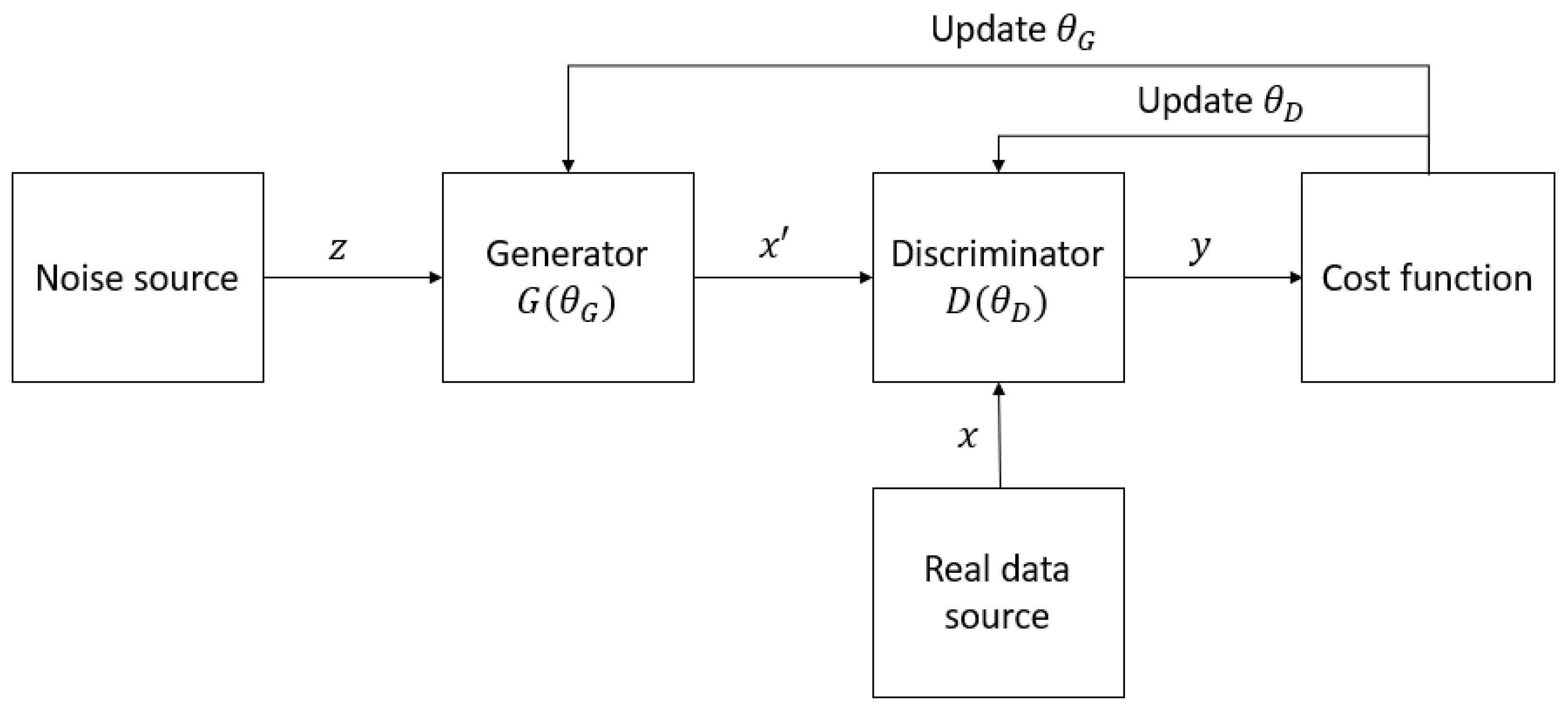
1.2. Quantum–Classical Interface
As quantum machines only work with data stored in quantum states, classical data must be encoded into this form of data. Therefore, data encoding (or embedding) has also become an interesting field of research. There are various data encoding techniques that are used in quantum machine learning algorithms, but in quantum GANs, basis encoding, amplitude encoding, and angle encoding are the most popular [60]. Basis encoding is the simplest way to embed classical data into a quantum state. The inputs must be in binary form, and each of them corresponds with a computational basis of the qubit system.23. Structures of QuGAN
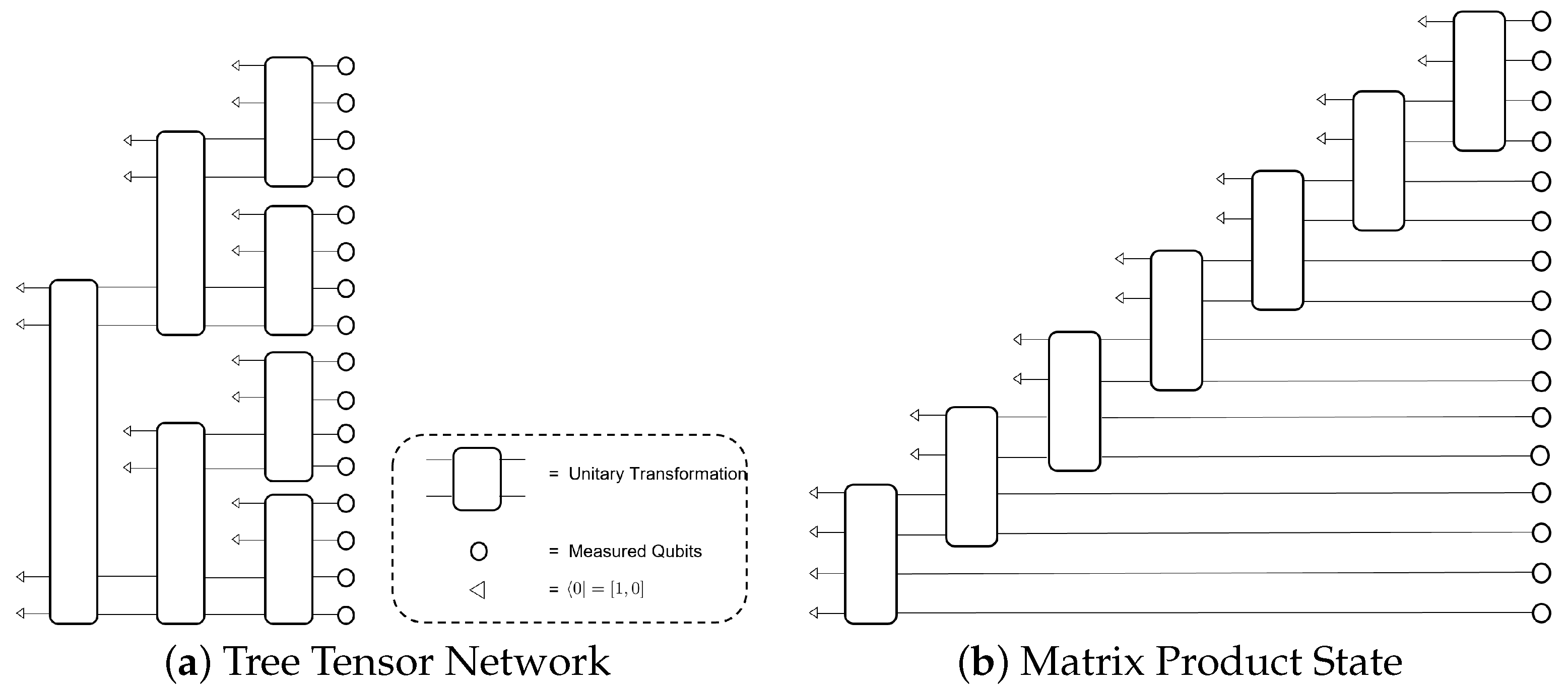
A QuGAN can be fully quantum, hybrid, or based on tensor networks. A diagram of quantum GAN categorization in terms of network architecture is sketched in Figure 2.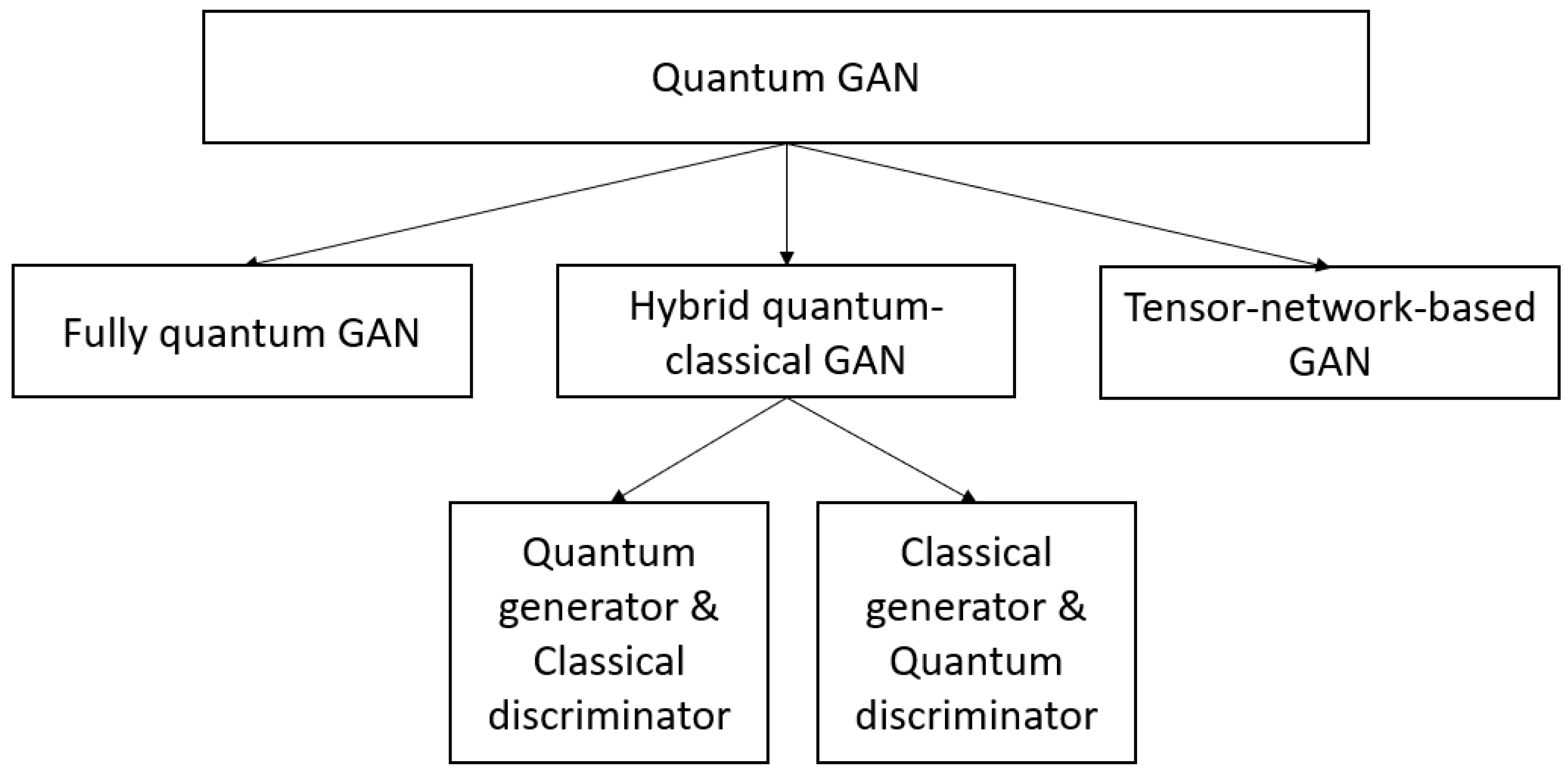
34. Optimization of QuGAN
34.1. Loss Function
Just like the traditional GANs, the quantum version needs a function whose gradients it can trace along to adjust its weight so as to reach the Nash equilibrium. This function may involve different quantities. Some QuGANs make use of the quantum states of the generator and the discriminator, and some others involve a certain function estimated by the discriminator (in this case, it is called the critic). However, in most QuGANs, the discriminating results of the discriminator are used to determine the loss.34.2. Gradient Computation
In quantum GANs, there are parametrized quantum circuits that build one or more parts of the network. That part can be the generator, or the discriminator, or both, or even the supplement components to assist the network in working more efficiently. These variational circuits consist of quantum gates or unitaries with tunable continuous parameters. Similarly to the classical counterparts, during the training process, the parameters are updated using a certain optimizing algorithm, such as gradient descent [61], Adam [62], or Adagrad [63]. All these approaches to adjusting the circuits to optimality require calculating the gradients of the cost function, including the partial derivatives with respect to the parameters of the circuits.34.3. Optimization and Evaluation Strategies
A good strategy to optimize a quantum GAN is also an important research direction with a lot of interesting questions. For example, what is the order of training the generator and the discriminator that results in the most efficient optimization process? How much should one train the generator in comparison with the discriminator? How many steps of gradients should the network go through? How can the parameters of a network be initialized for the best performance? Additionally, how can one set or even adjust the learning rate to adapt to the change during the training process? These problems matter when training a classical GAN, and they are certainly carried through to the quantum counterparts. With the exponential computational power and the more complicated algorithms, researchers should carefully set up the hyperparameters and determine the optimization strategy before conducting the training process. The solutions to these issues, however, are rather indiscriminate, and due to the different structures of the networks and the elusiveness of quantum nature, there has been no rule to find out the best training strategy that can be applied for every quantum network in general, and for every quantum GAN in particular. To tackle the learning rate and the number of measurement shots, Huang et al. [29] simply performed a grid search to find the optimal hyperparameters. In the same manner, some researchers also set the hyperparameters and adjust them manually during the training process.45. Quantum GAN Variants
45.1. Fully Quantum GANs
With fully quantum GANs, both generators and discriminators are constructed by quantum circuits, connected directly with the other, and they together apply to a system of qubits [27][28][29][64][65][66][67]. The target distributions can be quantum, which can be fed directly into the network, or classical, which must be encoded to some quantum states before being input into the network. The workflow of fully quantum GANs is depicted in Figure 3. The noise from latent space puts the quantum system in the state |z⟩. After being applied by the generator, the system is in state |ψ⟩. At this time, in the case the real data are used, the real quantum data source outputs state |x⟩ from the quantum system. The discriminator is then applied, and it changes the state to |y⟩. The states |y⟩ in the cases where the discriminator’s input is real or generated will then be used for the cost function and updating the parameters in the circuits.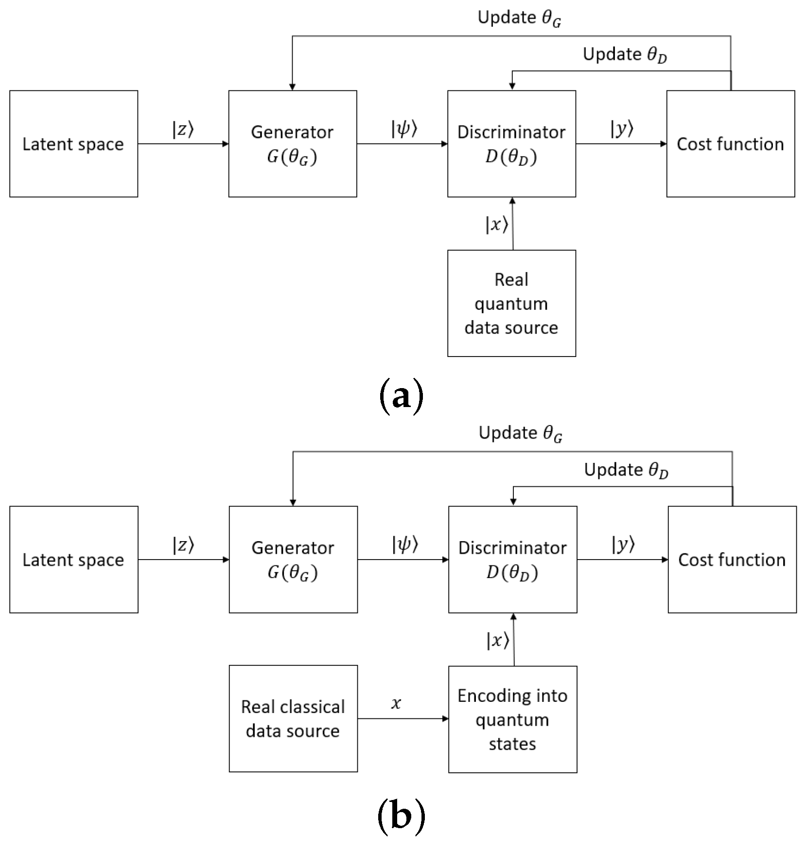
45.2. Hybrid Quantum–Classical GANs
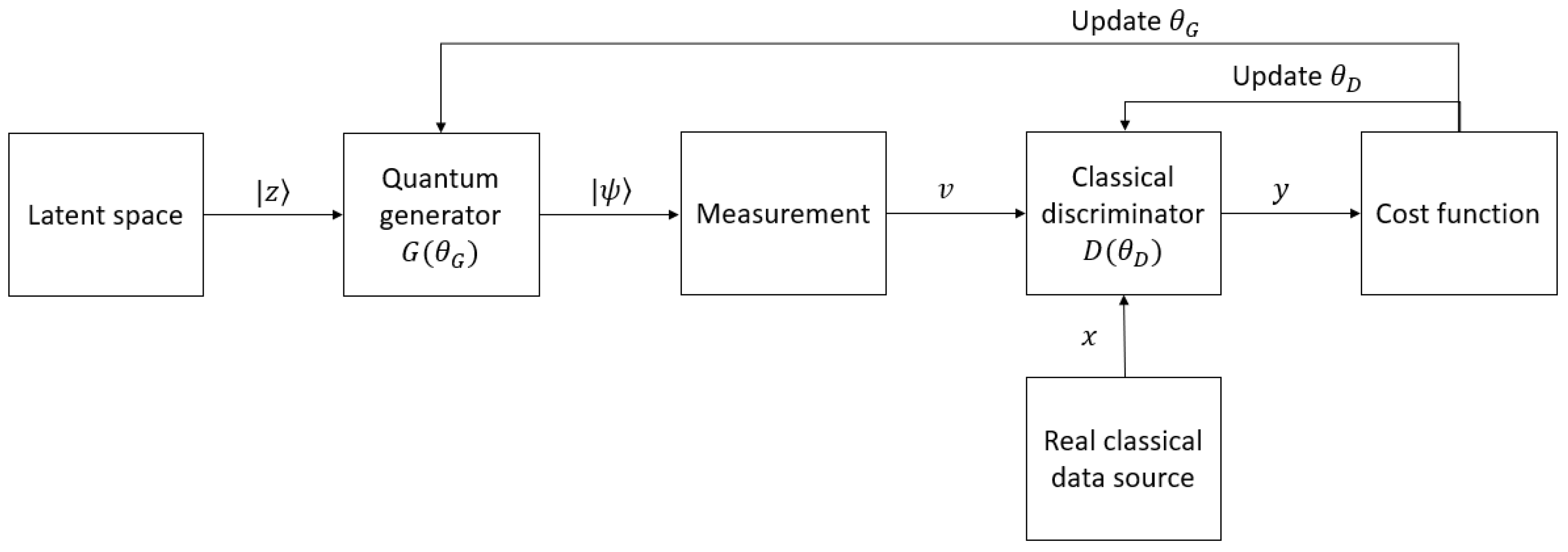
45.3. Tensor-Network-Based GANs
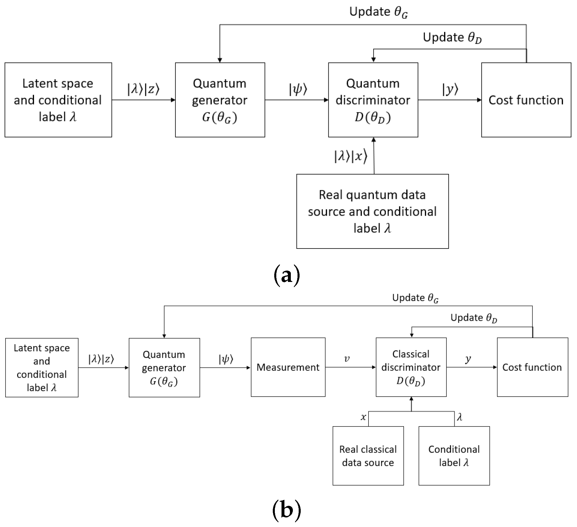
45.4. Quantum Conditional GANs
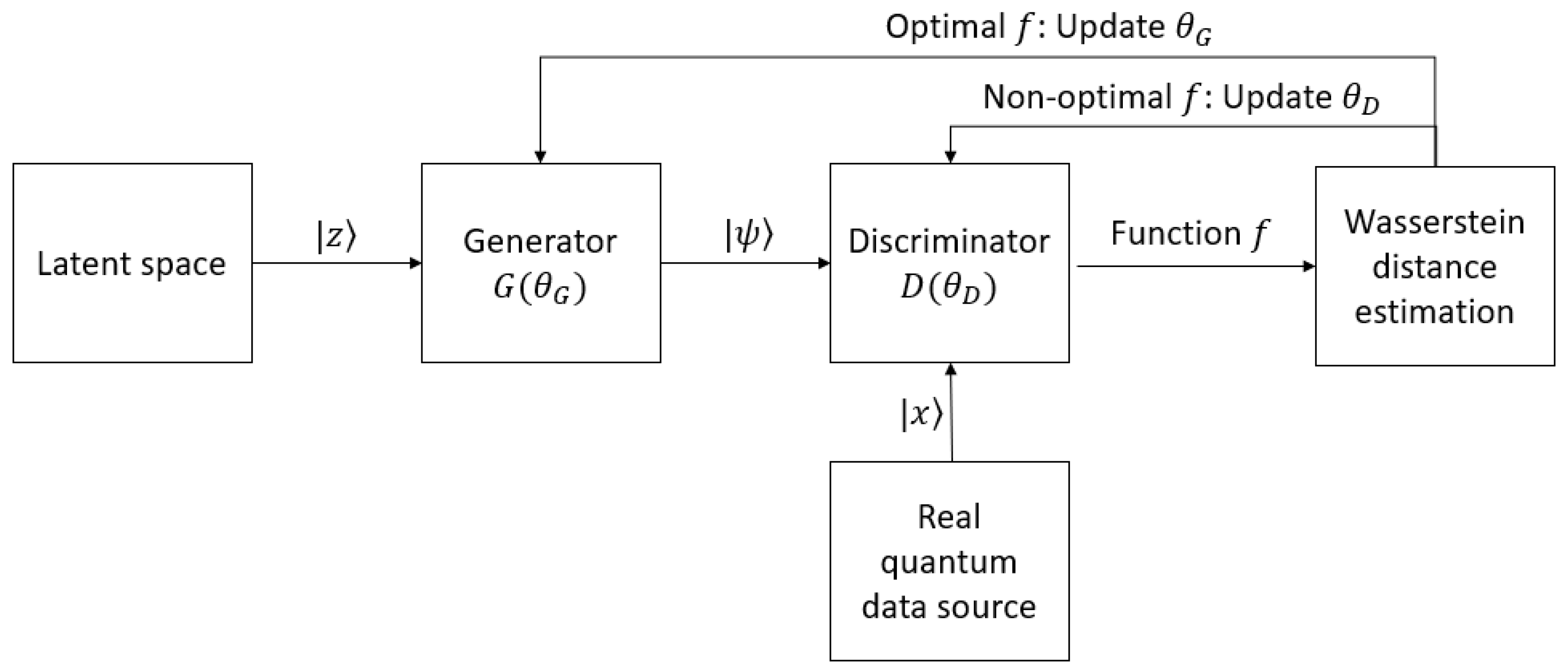
45.5. Quantum Wasserstein GANs
45.6. Quantum Patch GANs Using Multiple Sub-Generators
45.7. Quantum GANs Using Quantum Fidelity for a Cost Function
This fully quantum GAN variant was suggested by Stein et al. [28]. The architectures of the generator and the discriminator, the gradient calculation method, and the training strategy stay the same as other fully quantum GANs, but there is a modification in the cost function. The outcomes of the discriminator when the input is real (x) and fake (x′), i.e., D(x) and D(x'), are alternated by the fidelities of the state generated by encoding the real samples (ξ) and the state after applying by the generator (γ), respectively, with the state after applying the discriminator (δ).56. Conclusions
Quantum GAN is a new and potential field of research in quantum machine learning. This kind of quantum generative network is inspired by classical GANs, which have already proved their effectiveness and wide applications. In addition to the outstanding nature of GANs, quantum GANs even perform with higher efficiency due to their unique quantum properties and exponential computing power.References
- Mitchell, T.; Buchanan, B.; DeJong, G.; Dietterich, T.; Rosenbloom, P.; Waibel, A. Machine Learning. Annu. Rev. Comput. Sci. 1990, 4, 417–433.
- McCulloch, W.S.; Pitts, W. A logical calculus of the ideas immanent in nervous activity. Bull. Math. Biophys. 1943, 5, 115–133.
- Rosenblatt, F. The perceptron: A probabilistic model for information storage and organization in the brain. Psychol. Rev. 1958, 65, 386–408.
- Cortes, C.; Vapnik, V. Support-vector networks. Mach. Learn. 1995, 20, 273–297.
- Hopfield, J.J. Neural networks and physical systems with emergent collective computational abilities. Proc. Natl. Acad. Sci. USA 1982, 79, 2554–2558.
- LeCun, Y.; Bengio, Y.; Hinton, G. Deep Learning. Nature 2015, 521, 436–444.
- Alam, M.M.; Mohiuddin, K.; Das, A.K.; Islam, M.K.; Kaonain, M.S.; Ali, M.H. A Reduced Feature Based Neural Network Approach to Classify the Category of Students. In Proceedings of the 2nd International Conference on Innovation in Artificial Intelligence, Shanghai, China, 9–12 March 2018; Association for Computing Machinery: New York, NY, USA, 2018; pp. 28–32.
- Luckin, R.; Holmes, W.; Griffiths, M.; Forcier, L.B. Intelligence Unleashed: An Argument for AI in Education; Pearson Education: London, UK, 2016.
- Djambic, G.; Krajcar, M.; Bele, D. Machine learning model for early detection of higher education students that need additional attention in introductory programming courses. Int. J. Digit. Technol. Econ. 2016, 1, 1–11.
- Amatya, S.; Karkee, M.; Gongal, A.; Zhang, Q.; Whiting, M.D. Detection of cherry tree branches with full foliage in planar architecture for automated sweet-cherry harvesting. Biosyst. Eng. 2016, 146, 3–15.
- Pantazi, X.E.; Moshou, D.; Bravo, C. Active learning system for weed species recognition based on hyperspectral sensing. Biosyst. Eng. 2016, 146, 193–202.
- Bouri, E.; Gkillas, K.; Gupta, R.; Pierdzioch, C. Forecasting Realized Volatility of Bitcoin: The Role of the Trade War. Comput. Econ. 2021, 57, 29–53.
- Lussange, J.; Lazarevich, I.; Bourgeois-Gironde, S.; Palminteri, S.; Gutkin, B. Modelling Stock Markets by Multi-agent Reinforcement Learning. Comput. Econ. 2021, 57, 113–147.
- Sughasiny, M.; Rajeshwari, J. Application of Machine Learning Techniques, Big Data Analytics in Health Care Sector—A Literature Survey. In Proceedings of the 2018 2nd International Conference on I-SMAC (IoT in Social, Mobile, Analytics and Cloud) (I-SMAC), Palladam, India, 30–31 August 2018; pp. 741–749.
- Hazra, A.; Kumar, S.; Gupta, A. Study and Analysis of Breast Cancer Cell Detection using Naïve Bayes, SVM and Ensemble Algorithms. Int. J. Comput. Appl. 2016, 145, 39–45.
- Otoom, A.; Abdallah, E.; Kilani, Y.; Kefaye, A.; Ashour, M. Effective diagnosis and monitoring of heart disease. Int. J. Softw. Eng. Its Appl. 2015, 9, 143–156.
- Goodfellow, I.; Pouget-Abadie, J.; Mirza, M.; Xu, B.; Warde-Farley, D.; Ozair, S.; Courville, A.; Bengio, Y. Generative Adversarial Nets. In Advances in Neural Information Processing Systems; Ghahramani, Z., Welling, M., Cortes, C., Lawrence, N., Weinberger, K., Eds.; Curran Associates: New York, NY, USA, 2014; Volume 27.
- Farajzadeh-Zanjani, M.; Razavi-Far, R.; Saif, M.; Palade, V. Generative Adversarial Networks: A Survey on Training, Variants, and Applications. In Generative Adversarial Learning: Architectures and Applications; Razavi-Far, R., Ruiz-Garcia, A., Palade, V., Schmidhuber, J., Eds.; Springer International Publishing: Cham, Switzerland, 2022; pp. 7–29.
- Pradhyumna, P.; Mohana. A Survey of Modern Deep Learning based Generative Adversarial Networks (GANs). In Proceedings of the 2022 6th International Conference on Computing Methodologies and Communication (ICCMC), Erode, India, 29–31 March 2022; pp. 1146–1152.
- Preskill, J. Quantum Computing in the NISQ era and beyond. Quantum 2018, 2, 79.
- Harrow, A.W.; Montanaro, A. Quantum computational supremacy. Nature 2017, 549, 203–209.
- Biamonte, J.; Wittek, P.; Pancotti, N.; Rebentrost, P.; Wiebe, N.; Lloyd, S. Quantum machine learning. Nature 2017, 549, 195–202.
- Dong, D.; Chen, C.; Li, H.; Tarn, T.J. Quantum Reinforcement Learning. IEEE Trans. Syst. Man Cybern. Part B 2008, 38, 1207–1220.
- Rebentrost, P.; Mohseni, M.; Lloyd, S. Quantum Support Vector Machine for Big Data Classification. Phys. Rev. Lett. 2014, 113, 130503.
- Khoshaman, A.; Vinci, W.; Denis, B.; Andriyash, E.; Sadeghi, H.; Amin, M.H. Quantum variational autoencoder. Quantum Sci. Technol. 2018, 4, 14001.
- Lloyd, S.; Weedbrook, C. Quantum Generative Adversarial Learning. Phys. Rev. Lett. 2018, 121, 40502.
- Dallaire-Demers, P.L.; Killoran, N. Quantum generative adversarial networks. Phys. Rev. A 2018, 98, 12324.
- Stein, S.A.; Baheri, B.; Chen, D.; Mao, Y.; Guan, Q.; Li, A.; Fang, B.; Xu, S. QuGAN: A Quantum State Fidelity based Generative Adversarial Network. In Proceedings of the 2021 IEEE International Conference on Quantum Computing and Engineering (QCE), Broomfield, CO, USA, 17–22 October 2021; IEEE: Piscataway, NJ, USA, 2021.
- Huang, H.L.; Du, Y.; Gong, M.; Zhao, Y.; Wu, Y.; Wang, C.; Li, S.; Liang, F.; Lin, J.; Xu, Y.; et al. Experimental Quantum Generative Adversarial Networks for Image Generation. Phys. Rev. Appl. 2021, 16, 24051.
- Zoufal, C.; Lucchi, A.; Woerner, S. Quantum Generative Adversarial Networks for learning and loading random distributions. NPJ Quantum Inf. 2019, 5, 103.
- Krizhevsky, A.; Sutskever, I.; Hinton, G.E. ImageNet Classification with Deep Convolutional Neural Networks. In Advances in Neural Information Processing Systems; Pereira, F., Burges, C., Bottou, L., Weinberger, K., Eds.; Curran Associates: New York, NY, USA, 2012; Volume 25.
- Mirza, M.; Osindero, S. Conditional Generative Adversarial Nets. arXiv 2014, arXiv:1411.1784.
- Arjovsky, M.; Chintala, S.; Bottou, L. Wasserstein GAN. arXiv 2017, arXiv:1701.07875.
- Berthelot, D.; Schumm, T.; Metz, L. BEGAN: Boundary Equilibrium Generative Adversarial Networks. arXiv 2017, arXiv:1703.10717.
- Brock, A.; Donahue, J.; Simonyan, K. Large Scale GAN Training for High Fidelity Natural Image Synthesis. In Proceedings of the International Conference on Learning Representations, New Orleans, LA, USA, 6–9 May 2019.
- Denton, E.; Chintala, S.; Szlam, A.; Fergus, R. Deep Generative Image Models using a Laplacian Pyramid of Adversarial Networks. arXiv 2015, arXiv:1506.05751.
- Chen, X.; Duan, Y.; Houthooft, R.; Schulman, J.; Sutskever, I.; Abbeel, P. InfoGAN: Interpretable Representation Learning by Information Maximizing Generative Adversarial Nets. arXiv 2016, arXiv:1606.03657.
- Karras, T.; Aittala, M.; Laine, S.; Härkönen, E.; Hellsten, J.; Lehtinen, J.; Aila, T. Alias-Free Generative Adversarial Networks. arXiv 2021, arXiv:2106.12423.
- Tang, X.; Wang, Z.; Luo, W.; Gao, S. Face Aging with Identity-Preserved Conditional Generative Adversarial Networks. In Proceedings of the 2018 IEEE/CVF Conference on Computer Vision and Pattern Recognition, Salt Lake City, UT, USA, 18–23 June 2018; pp. 7939–7947.
- Wu, X.; Xu, K.; Hall, P. A survey of image synthesis and editing with generative adversarial networks. Tsinghua Sci. Technol. 2017, 22, 660–674.
- Dolhansky, B.; Ferrer, C.C. Eye In-Painting with Exemplar Generative Adversarial Networks. arXiv 2017, arXiv:1712.03999.
- Demir, U.; Unal, G. Patch-Based Image Inpainting with Generative Adversarial Networks. arXiv 2018, arXiv:1803.07422.
- Wu, H.; Zheng, S.; Zhang, J.; Huang, K. GP-GAN: Towards Realistic High-Resolution Image Blending. arXiv 2017, arXiv:1703.07195.
- Chen, B.C.; Kae, A. Toward Realistic Image Compositing With Adversarial Learning. In Proceedings of the 2019 IEEE/CVF Conference on Computer Vision and Pattern Recognition (CVPR), Long Beach, CA, USA, 15–20 June 2019; pp. 8407–8416.
- Wang, X.; Yu, K.; Wu, S.; Gu, J.; Liu, Y.; Dong, C.; Loy, C.C.; Qiao, Y.; Tang, X. ESRGAN: Enhanced Super-Resolution Generative Adversarial Networks. arXiv 2018, arXiv:1809.00219.
- Ding, Z.; Liu, X.Y.; Yin, M.; Kong, L. TGAN: Deep Tensor Generative Adversarial Nets for Large Image Generation. arXiv 2019, arXiv:1901.09953.
- Wang, C.; Xu, C.; Wang, C.; Tao, D. Perceptual Adversarial Networks for Image-to-Image Transformation. IEEE Trans. Image Process. 2018, 27, 4066–4079.
- Zhu, J.Y.; Park, T.; Isola, P.; Efros, A.A. Unpaired Image-to-Image Translation using Cycle-Consistent Adversarial Networks. arXiv 2017, arXiv:1703.10593.
- Liu, M.Y.; Breuel, T.; Kautz, J. Unsupervised Image-to-Image Translation Networks. arXiv 2017, arXiv:1703.00848.
- Kong, J.; Kim, J.; Bae, J. HiFi-GAN: Generative Adversarial Networks for Efficient and High Fidelity Speech Synthesis. arXiv 2020, arXiv:2010.05646.
- Oord, A.v.d.; Dieleman, S.; Zen, H.; Simonyan, K.; Vinyals, O.; Graves, A.; Kalchbrenner, N.; Senior, A.; Kavukcuoglu, K. WaveNet: A Generative Model for Raw Audio. arXiv 2016, arXiv:1609.03499.
- Dong, H.W.; Hsiao, W.Y.; Yang, L.C.; Yang, Y.H. MuseGAN: Multi-track Sequential Generative Adversarial Networks for Symbolic Music Generation and Accompaniment. arXiv 2017, arXiv:1709.06298.
- Engel, J.; Agrawal, K.K.; Chen, S.; Gulrajani, I.; Donahue, C.; Roberts, A. GANSynth: Adversarial Neural Audio Synthesis. arXiv 2019, arXiv:1902.08710.
- Uřičář, M.; Křížek, P.; Hurych, D.; Sobh, I.; Yogamani, S.; Denny, P. Yes, we GAN: Applying adversarial techniques for autonomous driving. Electron. Imaging 2019, 2019, 48-1–48-17.
- Jeong, C.H.; Yi, M.Y. Correcting rainfall forecasts of a numerical weather prediction model using generative adversarial networks. J. Supercomput. 2022, 79, 1289–1317.
- Besombes, C.; Pannekoucke, O.; Lapeyre, C.; Sanderson, B.; Thual, O. Producing realistic climate data with generative adversarial networks. Nonlinear Process. Geophys. 2021, 28, 347–370.
- Sandfort, V.; Yan, K.; Pickhardt, P.J.; Summers, R.M. Data augmentation using generative adversarial networks (CycleGAN) to improve generalizability in CT segmentation tasks. Sci. Rep. 2019, 9, 16884.
- Frid-Adar, M.; Diamant, I.; Klang, E.; Amitai, M.; Goldberger, J.; Greenspan, H. GAN-based synthetic medical image augmentation for increased CNN performance in liver lesion classification. Neurocomputing 2018, 321, 321–331.
- Cheng, J.; Yang, Y.; Tang, X.; Xiong, N.; Zhang, Y.; Lei, F. Generative Adversarial Networks: A Literature Review. KSII Trans. Internet Inf. Syst. 2020, 14, 4625–4647.
- Schuld, M. Supervised quantum machine learning models are kernel methods. arXiv 2021, arXiv:2101.11020.
- Lemaréchal, C. Cauchy and the gradient method. Doc. Math. Extra 2012, 251, 10.
- Kingma, D.P.; Ba, J. Adam: A Method for Stochastic Optimization. arXiv 2015, arXiv:1412.6980.
- Lydia, A.; Francis, S. Adagrad—An optimizer for stochastic gradient descent. Int. J. Inf. Comput. Sci 2019, 6, 566–568.
- Shrivastava, N.; Puri, N.; Gupta, P.; Krishnamurthy, B.; Verma, S. OpticalGAN: Generative Adversarial Networks for Continuous Variable Quantum Computation. arXiv 2019, arXiv:1909.07806.
- Hu, L.; Wu, S.H.; Cai, W.; Ma, Y.; Mu, X.; Xu, Y.; Wang, H.; Song, Y.; Deng, D.L.; Zou, C.L.; et al. Quantum generative adversarial learning in a superconducting quantum circuit. Sci. Adv. 2019, 5, eaav2761.
- Benedetti, M.; Grant, E.; Wossnig, L.; Severini, S. Adversarial quantum circuit learning for pure state approximation. New J. Phys. 2019, 21, 43023.
- Du, Y.; Hsieh, M.H.; Tao, D. Efficient Online Quantum Generative Adversarial Learning Algorithms with Applications. arXiv 2019, arXiv:1904.09602.
- Situ, H.; He, Z.; Wang, Y.; Li, L.; Zheng, S. Quantum generative adversarial network for generating discrete distribution. Inf. Sci. 2020, 538, 193–208.
- Huggins, W.; Patil, P.; Mitchell, B.; Whaley, K.B.; Stoudenmire, E.M. Towards quantum machine learning with tensor networks. Quantum Sci. Technol. 2019, 4, 24001.
- Han, Z.Y.; Wang, J.; Fan, H.; Wang, L.; Zhang, P. Unsupervised Generative Modeling Using Matrix Product States. Phys. Rev. X 2018, 8, 031012.
- Guo, C.; Jie, Z.; Lu, W.; Poletti, D. Matrix product operators for sequence-to-sequence learning. Phys. Rev. E 2018, 98, 042114.
