1.1. Generative Adversarial Networks (GANs)
The idea of quantum GANs originates from classical GANs, which were first proposed by Goodfellow et al.
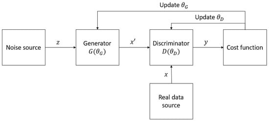
[17]. A GAN aims at learning a target distribution, which can be a series of text or a collection of images or audio, and generating samples that have similar characteristics to the samples in the training distribution. The architecture of a typical GAN is depicted in
Figure 1. A GAN typically consists of a generator
G and a discriminator
D. The generator and the discriminator are made from neural networks and are parameterized by
θG and
θD, respectively. The mission of
G is to take noise vectors
z from a noise source and produce data
x′ that mimic the realistic data
x as much as possible in order to fool
D, which is supposed to distinguish whether a sample is taken from the real distribution or is generated by
G. The distinguishing results
y of
D are then used to train both
G and
D iteratively; in other words,
θG and
θD are updated alternately until the network reaches its optimality. Ideally, this optimality, or Nash equilibrium
[17], occurs when
G can generate identical samples to those in the real distribution, and
D is not able to determine which source the data belong to.
Figure 1.
The architecture of a typical GAN.
GANs are the most potential and popular types of networks used for generative tasks. They vary in terms of network architectures, optimization strategies, and purposes of use. Some notable variants of GANs include deep convolutional GAN
[31][32], conditional GAN
[32][33], Wasserstein GAN
[33][34], boundary equilibrium GAN
[34][35], Big GAN
[35][36], Laplacian GAN
[36][37], and information maximizing GAN
[37][38]. Many GANs have been the basis of outstanding achievements. For example, StyleGAN3
[38][39] obtained a Fréchet inception distance of
3.07 on the FFHQ dataset,
4.40 on the AFHQv2 dataset, and
4.57 on the Beaches dataset. These networks have found their roles in image domains such as image synthesis
[35][36][39][40][36,37,40,41], image inpainting
[41][42][42,43], image blending
[43][44][44,45], image superresolution
[45][46][46,47], and image-to-image translation
[47][48][49][48,49,50]; audio domains such as speech synthesis
[50][51][51,52] and music composing
[52][53][53,54]; and other fields such as autonomous driving
[54][55], weather forecasting
[55][56][56,57], and data augmentation
[57][58][58,59]. GANs’ effectiveness and varied applications have been described in previous surveys of them
[18][19][59][18,19,60].
1.2. Quantum–Classical Interface
As quantum machines only work with data stored in quantum states, classical data must be encoded into this form of data. Therefore, data encoding (or embedding) has also become an interesting field of research. There are various data encoding techniques that are used in quantum machine learning algorithms, but in quantum GANs, basis encoding, amplitude encoding, and angle encoding are the most popular
[60][70]. Basis encoding is the simplest way to embed classical data into a quantum state. The inputs must be in binary form, and each of them corresponds with a computational basis of the qubit system.
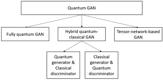
23. Structures of QuGAN
A QuGAN can be fully quantum, hybrid, or based on tensor networks. A diagram of quantum GAN categorization in terms of network architecture is sketched in
Figure 2.
Figure 2.
Quantum GAN structures.
In the fully quantum (or quantum-quantum) case, both the generator and the discriminator are quantum. Suppose the quantum generator produces fake data with a density matrix
ρ, and the quantum discriminator must discriminate those fake data with true data described by a density matrix
σ with a measurement operator
D. The outcomes of
D can be
T (i.e., true, or the data are from the real data source), or
F (i.e., false, or the data are generated by the generator). Since
T and
F are positive operators with a 1-norm less than or equal to 1, the set of them is convex, which means there must exist a minimum error measurement
[26]. To reach this optimal measurement, the discriminator aims to maximize the probability that it correctly categorizes the data as real or fake by following the gradients of the probability with respect to its parameters to adjust its weights. After that, due to the fact that the set of
ρ is convex, the generator also manages to adjust its own weights to maximize the probability that the discriminator fails to discriminate the data and produce an optimal density matrix
ρ [26]. Similarly to the traditional GANs, after a number of iterations of adjusting the weights of both the generator and the discriminator, a quantum GAN can also approach the Nash equilibrium.
The mechanism is similar when only a part of the classical GAN is replaced by a quantum engine. However, not all hybrid structures are possible. In particular, the generator or the discriminator cannot be classical if the training dataset is generated by a quantum system, which has quantum supremacy. This means the classical generator can never generate the statistics of a dataset that are similar to those of a quantum data source
[20]. Therefore, using the same strategy as in a fully quantum network, the quantum discriminator can always find a measurement to distinguish the true and the generated data. As a result, the probability that the discriminator makes wrong predictions will always be less than
12, and the Nash equilibrium will never happen
[26]. On the contrary, in the case where the discriminator is classical, both the real data and the generated data which are fed into the discriminator are quantum.
When the target data are classical, either the generator or the discriminator can be classical. However, although possessing quantum supremacy, the quantum systems only act on data as quantum states and are unable to work with classical data directly. If the discriminator is quantum, both the training data and the fake data generated by the classical generator need to be encoded before being fed into the discriminator. On the contrary, if the generator is quantum, the generated data must be measured using some computational bases to produce classical generated samples
[29][30][29,30].
34. Optimization of QuGAN
3.1. Loss Function
4.1. Loss Function
Just like the traditional GANs, the quantum version needs a function whose gradients it can trace along to adjust its weight so as to reach the Nash equilibrium. This function may involve different quantities. Some QuGANs make use of the quantum states of the generator and the discriminator, and some others involve a certain function estimated by the discriminator (in this case, it is called the critic). However, in most QuGANs, the discriminating results of the discriminator are used to determine the loss.
3.2. Gradient Computation
4.2. Gradient Computation
In quantum GANs, there are parametrized quantum circuits that build one or more parts of the network. That part can be the generator, or the discriminator, or both, or even the supplement components to assist the network in working more efficiently. These variational circuits consist of quantum gates or unitaries with tunable continuous parameters. Similarly to the classical counterparts, during the training process, the parameters are updated using a certain optimizing algorithm, such as gradient descent
[61][88], Adam
[62][89], or Adagrad
[63][90]. All these approaches to adjusting the circuits to optimality require calculating the gradients of the cost function, including the partial derivatives with respect to the parameters of the circuits.
3.3. Optimization and Evaluation Strategies
4.3. Optimization and Evaluation Strategies
A good strategy to optimize a quantum GAN is also an important research direction with a lot of interesting questions. For example, what is the order of training the generator and the discriminator that results in the most efficient optimization process? How much should one train the generator in comparison with the discriminator? How many steps of gradients should the network go through? How can the parameters of a network be initialized for the best performance? Additionally, how can one set or even adjust the learning rate to adapt to the change during the training process?
These problems matter when training a classical GAN, and they are certainly carried through to the quantum counterparts. With the exponential computational power and the more complicated algorithms, researchers should carefully set up the hyperparameters and determine the optimization strategy before conducting the training process.
The solutions to these issues, however, are rather indiscriminate, and due to the different structures of the networks and the elusiveness of quantum nature, there has been no rule to find out the best training strategy that can be applied for every quantum network in general, and for every quantum GAN in particular. To tackle the learning rate and the number of measurement shots, Huang et al.
[29] simply performed a grid search to find the optimal hyperparameters. In the same manner, some researchers also set the hyperparameters and adjust them manually during the training process.
45. Quantum GAN Variants
4.1. Fully Quantum GANs
5.1. Fully Quantum GANs
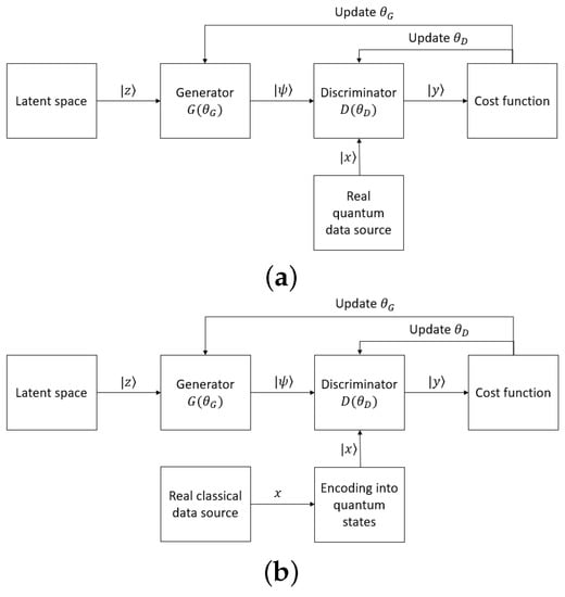
With fully quantum GANs, both generators and discriminators are constructed by quantum circuits, connected directly with the other, and they together apply to a system of qubits
[27][28][29][64][65][66][67][27,28,29,79,86,87,93]. The target distributions can be quantum, which can be fed directly into the network, or classical, which must be encoded to some quantum states before being input into the network. The workflow of fully quantum GANs is depicted in
Figure 34. The noise from latent space puts the quantum system in the state
|z⟩. After being applied by the generator, the system is in state
|ψ⟩. At this time, in the case the real data are used, the real quantum data source outputs state
|x⟩ from the quantum system. The discriminator is then applied, and it changes the state to
|y⟩. The states
|y⟩ in the cases where the discriminator’s input is real or generated will then be used for the cost function and updating the parameters in the circuits.
Figure 34.
The workflow of a fully quantum network in the cases where the target data are (
a
) quantum and (
b
) classical.
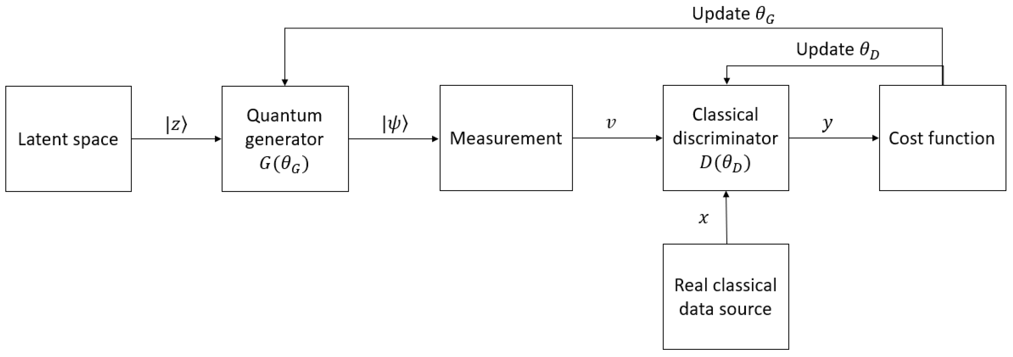
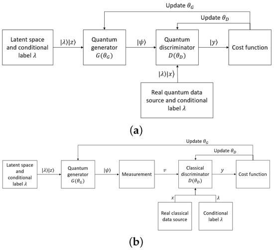
4.2. Hybrid Quantum–Classical GANs
5.2. Hybrid Quantum–Classical GANs
A GAN could be a combination of a quantum and a classical module. In practice, a GAN with a classical generator and a quantum discriminator is never used. As stated in
[26], if the target distribution is quantum, it is impossible for the classical generator to estimate and learn such a distribution. On the other hand, if the target data are classical, the generator is able to generate such data, but it can always be beaten by the quantum discriminator. In this way, the generator never reaches its convergence. Hence, a hybrid quantum–classical GAN has a quantum generator and a classical discriminator. The architecture of a hybrid quantum–classical GAN is illustrated in
Figure 45. This variant of quantum GANs is used to generate classical data with extraordinary performance in comparison with traditional GANs. Since the discriminator is also classical, the target data do not need encoding. However, the states of the quantum system after the generator must be measured to be transformed into classical statistics, which are readable for the discriminator. The classical discriminator can be made of a fully connected neural network
[29][30][68][29,30,80], with its output being 0 or 1, corresponding with real and fake examples, respectively.
Figure 45.
The workflow of a hybrid quantum–classical GAN.
4.3. Tensor-Network-Based GANs
5.3. Tensor-Network-Based GANs
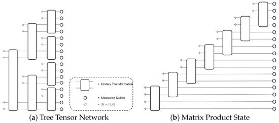
Tensor networks have recently been considered as a promising design for many generative learning tasks
[69][70][71][76,97,98]. In
[69][76], the authors considered two families of tensor networks, namely, matrix product states and tree tensor networks, to model a generative circuit. Their architectures are shown in
Figure 56. Rather than applying the universal unitary operators of all qubits, tensor-network-based generative models consider some specific patterns by choosing a subset of qubits for each unitary transformation. The algorithms begin by initializing 2V qubits in one subset in a reference computational basis state
⟨0|⊗2V , then transform these qubits by a unitary operator. Another subset of 2V qubits is prepared in
⟨0|⊗2V, and half of them will be entangled with V qubits from the first subset by another unitary operator. The process continues until the total number of qubits reaches the desired output dimensionality.
Figure 56 shows examples of the designs of generators based on tree tensor network (a) and matrix product states (b) with V = 2.
Figure 56.
Generative models with tensor networks.
4.4. Quantum Conditional GANs
5.4. Quantum Conditional GANs
In classical generative tasks, the input of the generator is random, so one has no control over the generated output. To force the network to produce the examples with desired classes, one conditional constraint about the label is added
[32][33]. Both the generator and the discriminator are aware of this constraint. In addition to discriminating whether the sample comes from a real or generated distribution, the discriminator has to evaluate whether the sample has the characteristics corresponding to the right label or not. This is the same approach when it comes to the quantum scenario. The conditional label
λ is also encoded in the form of quantum states. The schematic of quantum conditional GANs is shown in
Figure 67.
Figure 67. The workflow of (
a) a quantum conditional GAN generating quantum data and (
b) that of a hybrid conditional GAN generating classical data.
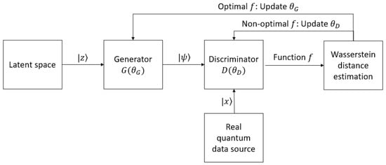
4.5. Quantum Wasserstein GANs
5.5. Quantum Wasserstein GANs
Quantum Wasserstein GANs are the quantum GANs that use Wasserstein distance, or Earth mover’s distance (EMD), as their cost functions. Differently from other quantum GANs variants, the mission of the discriminator in Wasserstein GANs (WGANs) is not to distinguish between the real and the generated data. Due to the fact that Wasserstein distance contains a function that satisfies the Lipschitz condition, the discriminator acts as an estimator that finds out the optimal function for calculating the distance. After the distance is computed, it is used to update the parameters in the generator. The workflow of quantum WGANs is illustrated in
Figure 78.
Figure 78.
The general workflow of a quantum WGAN.
4.6. Quantum Patch GANs Using Multiple Sub-Generators
5.6. Quantum Patch GANs Using Multiple Sub-Generators
For a classical dataset with
M dimensions, whichever encoding method is used, each sample requires at least
N=logM qubits to be represented. To deal with the case there are limited quantum resources, i.e., the number of available qubits, Huang et al. suggested a quantum patch GAN
[29]. This network consists of
T quantum sub-generators and a classical discriminator. The sub-generators are identical, and each is responsible for a portion of the high-dimensional data. The outputs of the sub-generators are measured and concatenated together to form a classical vector, which then can be fed into the discriminator. Thanks to dividing the data into small parts for each sub-generator, the training can be carried out on distributed quantum devices parallelly or on a single quantum device sequentially.
4.7. Quantum GANs Using Quantum Fidelity for a Cost Function
5.7. Quantum GANs Using Quantum Fidelity for a Cost Function
This fully quantum GAN variant was suggested by Stein et al.
[28]. The architectures of the generator and the discriminator, the gradient calculation method, and the training strategy stay the same as other fully quantum GANs, but there is a modification in the cost function. The outcomes of the discriminator when the input is real
(x) and fake
(x′), i.e.,
D(x) and
D(x'), are alternated by the fidelities of the state generated by encoding the real samples (
ξ) and the state after applying by the generator (
γ), respectively, with the state after applying the discriminator (
δ).
56. Conclusions
Quantum GAN is a new and potential field of research in quantum machine learning. This kind of quantum generative network is inspired by classical GANs, which have already proved their effectiveness and wide applications. In addition to the outstanding nature of GANs, quantum GANs even perform with higher efficiency due to their unique quantum properties and exponential computing power.