Your browser does not fully support modern features. Please upgrade for a smoother experience.
Submitted Successfully!
 +1 credit
Thank you for your contribution! You can also upload a video entry or images related to this topic.
For video creation, please contact our Academic Video Service.
| Version | Summary | Created by | Modification | Content Size | Created at | Operation |
|---|---|---|---|---|---|---|
| 1 | Tomasz Praczyk | -- | 2382 | 2022-08-15 09:28:05 | | | |
| 2 | Catherine Yang | + 1 word(s) | 2383 | 2022-08-15 09:46:32 | | | | |
| 3 | Catherine Yang | Meta information modification | 2383 | 2022-08-15 09:49:58 | | |
Video Upload Options
We provide professional Academic Video Service to translate complex research into visually appealing presentations. Would you like to try it?
Cite
If you have any further questions, please contact Encyclopedia Editorial Office.
Praczyk, T. Hill Climb Assembler Encoding. Encyclopedia. Available online: https://encyclopedia.pub/entry/26142 (accessed on 25 July 2026).
Praczyk T. Hill Climb Assembler Encoding. Encyclopedia. Available at: https://encyclopedia.pub/entry/26142. Accessed July 25, 2026.
Praczyk, Tomasz. "Hill Climb Assembler Encoding" Encyclopedia, https://encyclopedia.pub/entry/26142 (accessed July 25, 2026).
Praczyk, T. (2022, August 15). Hill Climb Assembler Encoding. In Encyclopedia. https://encyclopedia.pub/entry/26142
Praczyk, Tomasz. "Hill Climb Assembler Encoding." Encyclopedia. Web. 15 August, 2022.
Copy Citation
Hill Climb Assembler Encoding (HCAE) which is a light variant of Hill Climb Modular Assembler Encoding (HCMAE). While HCMAE, as the name implies, is dedicated to modular neural networks, the target application of HCAE is to evolve small/mid-scale monolithic neural networks. HCAE is a light variant of HCMAE and it originates from both AE and AEEO. All the algorithms are based on three key components, i.e., a network definition matrix (NDM), which represents the neural networks, assembler encoding program (AEP), which operates on NDM, and evolutionary algorithm, whose task is to produce optimal AEPs, NDMs, and, consequently, the networks.
evolutionary neural networks
hill climb
control
1. Network Definition Matrix
To represent a neural network, HCAE, like its predecessors, uses a matrix called network definition matrix (NDM). The matrix includes all the parameters of the network, including the weights of inter-neuron connections, bias, etc. The matrix which contains non-zero elements above and below the diagonal encodes a recurrent neural network (RANN), whereas the matrix with only the content above the diagonal represents a feed-forward network (FFANN) [1].
2. Assembler Encoding Program
In all the AE family, filling up the matrix, and, consequently, constructing an ANN is the task of an assembler encoding program (AEP) which, like an assembler program, consists of a list of operations and a sequence of data. Each operation implements a fixed algorithm and its role is to modify a piece of NDM. The operations are run one after another and their working areas can overlap, which means that modifications made by one operation can be overwritten by other operations which are placed further in the program. AEPs can be homogeneous or heterogeneous in terms of applied operations. In the first case, all operations in AEP are of the same type and they implement the same algorithm whereas, in the second case, AEPs can include operations with different algorithms. The first solution is applied in HCAE and AEEO, whereas the second one in AE [1].
The way each operation works depends, on the one hand, on its algorithm and, on the other hand, on its parameters. Each operation can be fed with its “private” parameters, linked exclusively to it, or with a list of shared parameters concentrated in the data sequence. Parametrization allows operations with the same algorithm to work in a different manner, for example, to work in different fragments of NDM.
HCAE uses two types of operations, say, Oper1 and Oper2. Oper1 is an adaptation of a solution applied in AEEO. It is of a global range, which means that it can modify any element of NDM, and it uses a small feed-forward neural network, say, ANN operation, in the decision-making process. The task of ANN operation is to decide which NDM items are to be updated and how they are to be updated (see Figure 1). The architecture of each ANN operation is determined by parameters of Oper1, whereas inputs to the ANN operation are taken from the data sequence of AEP. A pseudo-code of Oper1 is given in Algorithm 1.
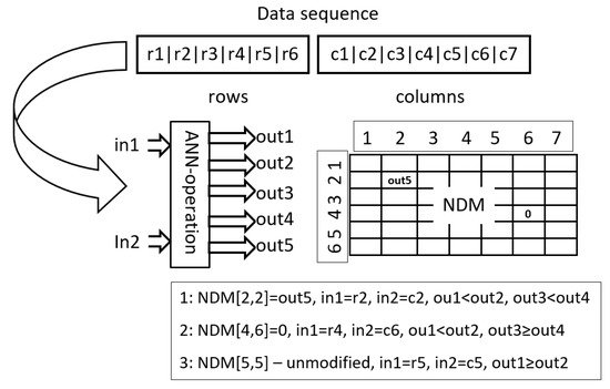
Figure 1. Applying ANN operations in Oper1: ANN operation is run for each item in NDM, one after another, and it can change the value of each item. The figure shows applying the network to determine the value of three items: NDM[2,2], NDM[4,6] and NDM[5,5]. In the first case, the item is modified to the value out5, which is the response of the network to the input r2,c2. r2,c2 are data items that correspond to the second row and column, that is, to the location of the modified item. The value out5 is inserted into NDM because out1<out2 and out3<out4. In the second case, the item receives the value 0 because out1<out2 and out3≥out4. In addition, in the third case, the item is left unchanged because out1≥out2.
Each ANN operation has two inputs and five outputs. The inputs indicate individual items of NDM. In AEEO, ANN operations are fed with coordinates of items to be modified, that is, with numbers of columns and rows, for example, in order to modify item [i,j], an ANN operation is supplied with i and j. In HCAE, a different approach is used, namely, instead of i, j, ANN operations are fed with data items which correspond to i and j, that is, with row [i] and column [j] (lines (10) and (11) in Algorithm 1). Vectors row and column are filled with appropriate data items (lines (2) and (5) in Algorithm 1).
The outputs of ANN operation decide whether to modify a given item of NDM or to leave it intact—outputs no. 1 and no. 2 (line (13) in Algorithm 1), and then, whether to reset the item or to assign it a new value—outputs no. 3 and no. 4 (line (14) in Algorithm 1), the new value is taken from the fifth output of the ANN operation (line (15) in Algorithm 1). Parameter M is a scaling parameter.
| Algorithm 1 Pseudo-code of Oper1. |
| Input: operation parameters (p), data sequence (d), NDM Output: NDM 1: for i∈<0..NDM.numberOfRows) do 2: row[i] ← d[i mod d.length]; 3: end for 4: for i∈<0..NDM.numberOfColumns) do 5: column[i] ← d[(i+NDM.numberOfRows) mod d.length]; 6: end for 7: ANN-oper ← getANN(p); 8: fori∈<0..NDM.numberOfColumns) do 9: for j∈<0..NDM.numberOfRows) do 10: ANN-oper.setIn(1,row[j]); 11: ANN-oper.setIn(2,column[i]); 12: ANN-oper.run(); 13: if ANN-oper.getOut(1) <ANN-oper.getOut(2) then 14: if ANN-oper.getOut(3) < ANN-oper.getOut(4) then 15: NDM[j,i] ←M*ANN-oper.getOut(5); 16: else 17: NDM[j,i] ← 0; 18: end if 19: end if 20: end for 21: end for 22: Return NDM |
Like resultant ANNs, ANN operations are also represented in the form of NDMs, say, NDM operations. To generate an NDM operation, and consequently, an ANN operation, getANN(p) is applied whose pseudo-code is depicted in Algorithm 2. It fills all matrix items with subsequent parameters of Oper1 divided by a scaling coefficient, N. If the number of parameters is too small to fill the entire matrix, they are used many times.
| Algorithm 2 Pseudo-code of getANN. |
| Input: operation parameters (p) Output: ANN-operation 1: NDM-operation ← 0; 2: noOfItem← 0; 3: for i∈<0..NDM-operation.numberOfColumns) do 4: for j<i //feed-forward ANN do 5: NDM-operation[j,i] ← p[noOfItemmod p.length]/N; 6: noOfItem++; 7: end for 8: end for 9: Return ANN-operation encoded in NDM-operation. |
Unlike Oper1, Oper2 works locally in NDM, and is an adaptation of a solution applied in AE. Pseudo-code of Oper2 is given in Algorithm 3 and 4. It does not use ANN-operations; instead, it directly fills NDM with values from the data sequence of AEP: where NDM is updated, and which and how many data items are used, are determined by operation parameters. The first parameter indicates the direction according to which NDM is modified, that is, whether it is changed along columns or rows (lines (4) and (10) in Algorithm 3). The second parameter determines the size of holes between NDM updates, that is, the number of zeros that separate consecutive updates (line (3) in Algorithm 4). The next two parameters point out the location in NDM where the operation starts to work, i.e., they indicate the starting row and column (line (1) in Algorithm 4). The fifth parameter determines the size of the altered NDM area, in other words, it indicates how many NDM items are updated (line (1) in Algorithm 4). Additionally, the last, sixth parameter points out location in the sequence of data from where the operation starts to take data items and put them into the NDM (line (2) in Algorithm 3) [1].
| Algorithm 3 Pseudo-code of Oper2 [1]. |
| Input: operation parameters (p), data sequence (d), NDM Output: NDM 1: filled← 0; 2: where← p[6]; 3: holes← 0; 4: if p[1] mod 2 = 0 then 5: for k∈<0..NDM.numberOfColumns) do 6: for j∈<0..NDM.numberOfRows) do 7: NDM[j,k] ← fill(k,j,param,data,filled,where,holes); 8: end for 9: end for 10: else 11: for k∈<0..NDM.numberOfRows) do 12: for j∈<0..NDM.numberOfColumns) do 13: NDM[k,j] ← fill(j,k,p,d,filled,where,holes); 14: end for 15: end for 16: end if 17: Return NDM. |
| Algorithm 4 Pseudo-code of fill () [1]. |
| Input: number of column (c), number of row (r), operation parameters (p), data sequence (d), number of updated items (f), starting position in data (w), number of holes (h) Output: new value for NDM item 1: if f < p[5] and c ≥ p[4] andr≥ p[3] then 2: f++; 3: if h = p[2] then 4: h ← 0; 5: w++; 6: Return d[w mod d.length]; 7: else 8: h++; 9: Return 0. 10: end if 11: end if |
3. Evolutionary Algorithm
The common characteristic of all AE-based algorithms is the use of cooperative co-evolutionary GA (CCEGA) [2][3] to evolve AEPs, that is, to determine the number of operations (AE,AEEO), the type of each operation (AE), the parameters of the operations (all algorithms), the length of the data sequence (AE,AEEO), and its content (all algorithms). As already mentioned, the implementations of operations are predefined. According to CCEGA, each evolved component of AEP evolves in a separate population, that is, an AEP with n operations and the sequence of data evolves in n+1 populations (see Figure 2) [1].
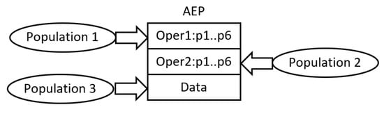
Figure 2. Evolution of AEPs according to CCEGA
To construct a complete AEP, NDM, and finally, a network, the operations and the data are combined together according to the procedure applied in CCEGA. An individual (for example, an operation) from an evaluated population is linked to the best leader individuals from the remaining populations that evolved in all previous CCEGA iterations. Each population maintains the leader individuals, which are applied as building blocks of all AEPs constructed during the evolutionary process. In order to evaluate newborn individuals, they are combined with the leader individuals from the remaining populations [1].
Even though all the AE family applies CCEGA to evolve neural networks, HCAE does it in a different way from the remaining AE algorithms. In AE/AEEO, the networks evolve in one potentially infinite loop of CCEGA. Throughout the evolution, AEPs can grow or shrink, that is, they adjust their complexity to the task by changing in size. Each growth or shrinkage entails a change in the number of populations in which AEPs evolve. Unfortunately, such an approach appeared to be ineffective for a greater number of operations/populations. Usually, an increase in the number of operations/populations to three or more does not improve results, which is due to the difficulties in the coordination of a greater number of operations.
In contrast to AE/AEEO, HCAE is a hill climber whose each step is made by CCEGA (see Algorithm 5). A starting point of the algorithm is a blank network represented by a blank NDM (line (1)). Then, the network as well as NDM are improved in subsequent evolutionary runs of CCEGA (line (5)). Each next run works on the best network/NDM found so far by all earlier runs (each AEP works on its own copy of NDM), is interrupted after a specified number of iterations without progress (MAX_ITER_NO_PROG), and delegates outside, to the HCAE main loop, the best network/NDM that evolved within the run (tempNDM). If this network/NDM is better than those generated by earlier CCEGA runs, a next HCAE step is made—each subsequent network/NDM has to be better than its predecessor (line (7) [1] ).
| Algorithm 5 Evolution in HCAE [1]. |
| Input: CCEGA parameters, for example crossover probability Output: Neural network 1: NDM ← 0; 2: numberOfIter← 0; 3: fitness← evaluation of NDM; 4: while numberOfIter < maxEval and fitness < acceptedFitnessdo 5: tempNDM ← CCEGA.run(NDM,MAX_ITER_NO_PROG); 6: if tempNDM.fitness > fitness then 7: NDM ← tempNDM; 8: fitness ← tempNDM.fitness; 9: end if 10: numberOfIter ← numberOfIter + 1; 11: end while 12: Return Neural network decoded from NDM. |
In order to avoid AE/AEEO problems with the effective processing of complex AEPs, HCAE uses constant-length programs of a small size. They include, at most, two operations and the sequence of data; the number of operations does not change over time. Such a construction of AEPs affects the structure of CCEGA. In this case, AEPs evolve in two or, at most, three populations; the number of populations is invariable. One population includes sequences of data, i.e., chromosomes data, whereas the remaining populations contain encoded operations, i.e., chromosomes operations. The operations are encoded as integer strings, whereas the data as real-valued vectors, which is a next difference between HCAE and AE/AEEO that apply binary encoding. Both chromosomes operations and chromosomes data are of constant length.
In HCAE, like in AE/AEEO, the evolution in all the populations takes place according to simple canonical genetic algorithm with a tournament selection. The chromosomes undergo two classical genetic operators, i.e., one-point crossover and mutation. The crossover is performed with a constant probability Pc, whereas the mutation is adjusted to the current state of the evolutionary process. Its probability (Pdm—probability of mutation in data sequences; Pom—probability of mutation in operations) grows once there is no progress for a time and it decreases once progress is noticed [1].
The chromosomes data and chromosomes operations are mutated differently, and they are performed according to Equations (1) and (2) [1].
where d—is a gene in a chromosome-data; o—is a gene in a chromosome-operation; randU(−a,a)—is a uniformly distributed random real value from the range <−a,a>; randI(−b,b)—is a uniformly distributed random integer value from the range <−b,b>; Po,zerom—is a probability of a mutated gene to be zero.
4. Complexity Analysis
Although algorithms no. 1, 2 and 3 present the traditional iterative implementation style, which is due to the ease of analysis of such algorithms, the actual HCAE implementation is parallel. This means that the algorithm can be divided into three parallel blocks executed one after the other, namely: the genetic algorithm (CCEGA + CGA), the AEP program and the evaluation of neural networks. The complexity of the algorithm can therefore be defined as O(O(CCEGA + CGA) + O(AEP) + O(Fitness)). The parallel implementation of the genetic algorithm requires, in principle, three steps, i.e., selection of parent individuals, crossover and mutation, which means that the researchers obtain O(3). In addition, it also requires l(n+n1n2) processors or processor cores, where l is the number of chromosomes in a single CCEGA population, n1 is the number of AEP operations, and n and n2 are the number of genes in chromosome data and chromosomes operations, respectively. The AEP program is executed in n1 steps (O(n1)) and requires a maximum of Z processors/cores, where Z is the number of cells of the NDM matrix. The last block of the algorithm is the evaluation of neural networks, the computational complexity of which depends on the problem being solved. Ignoring the network evaluation, it can be concluded that the algorithm complexity is O(3 + n1) and requires max(l(n+n1n2),Z) processors/cores.
References
- Praczyk, T. Hill Climb Modular Assembler Encoding: Evolving Modular Neural Networks of fixed modular architecture. Knowl.-Based Syst. 2022, 232.
- Potter, M. The Design and Analysis of a Computational Model of Cooperative Coevolution. Ph.D. Thesis, George Mason University, Fairfax, VA, USA, 1997.
- Potter, M.A.; Jong, K.A.D. Cooperative coevolution: An architecture for evolving coadapted subcomponents. Evol. Comput. 2000, 8, 1–29.
More
Information
Contributor
MDPI registered users' name will be linked to their SciProfiles pages. To register with us, please refer to https://encyclopedia.pub/register
:
View Times:
741
Revisions:
3 times
(View History)
Update Date:
15 Aug 2022
Table of Contents


Notice
You are not a member of the advisory board for this topic. If you want to update advisory board member profile, please contact office@encyclopedia.pub.
OK
Confirm
Only members of the Encyclopedia advisory board for this topic are allowed to note entries. Would you like to become an advisory board member of the Encyclopedia?
Yes
No
${ textCharacter }/${ maxCharacter }
Submit
Cancel
Back
Comments
${ item }
|
${ item.createdUser.fullName }
${ item.createdAt }
${ item.vote }
${ item.reply }
Delete
${ reply.createdUser.fullName }
${ reply.createdAt }
${ reply.vote }
Delete
There is no reply to this comment~
${ item.replyTextCharacter }/${ item.replyMaxCharacter }
Submit
Cancel
More
No more~
There is no comment~
${ textCharacter }/${ maxCharacter }
Submit
Cancel
${ selectedItem.replyTextCharacter }/${ selectedItem.replyMaxCharacter }
Submit
Cancel
Confirm
Are you sure to Delete?
Yes
No