Your browser does not fully support modern features. Please upgrade for a smoother experience.
Submitted Successfully!
 +1 credit
Thank you for your contribution! You can also upload a video entry or images related to this topic.
For video creation, please contact our Academic Video Service.
| Version | Summary | Created by | Modification | Content Size | Created at | Operation |
|---|---|---|---|---|---|---|
| 1 | Luz del Carmen García Rodríguez | -- | 3258 | 2022-06-21 14:28:37 | | | |
| 2 | Conner Chen | -3 word(s) | 3255 | 2022-06-22 10:26:20 | | | | |
| 3 | Conner Chen | Meta information modification | 3255 | 2022-06-22 10:35:36 | | |
Video Upload Options
We provide professional Academic Video Service to translate complex research into visually appealing presentations. Would you like to try it?
Cite
If you have any further questions, please contact Encyclopedia Editorial Office.
García-Rodríguez, L.D.C.; Prado-Olivarez, J.; Guzmán-Cruz, R.; Rodríguez-Licea, M.A.; Barranco-Gutiérrez, A.I.; Perez-Pinal, F.J.; Espinosa-Calderon, A. Mathematical Modeling to Estimate Photosynthesis. Encyclopedia. Available online: https://encyclopedia.pub/entry/24281 (accessed on 06 June 2026).
García-Rodríguez LDC, Prado-Olivarez J, Guzmán-Cruz R, Rodríguez-Licea MA, Barranco-Gutiérrez AI, Perez-Pinal FJ, et al. Mathematical Modeling to Estimate Photosynthesis. Encyclopedia. Available at: https://encyclopedia.pub/entry/24281. Accessed June 06, 2026.
García-Rodríguez, Luz Del Carmen, Juan Prado-Olivarez, Rosario Guzmán-Cruz, Martín Antonio Rodríguez-Licea, Alejandro Israel Barranco-Gutiérrez, Francisco Javier Perez-Pinal, Alejandro Espinosa-Calderon. "Mathematical Modeling to Estimate Photosynthesis" Encyclopedia, https://encyclopedia.pub/entry/24281 (accessed June 06, 2026).
García-Rodríguez, L.D.C., Prado-Olivarez, J., Guzmán-Cruz, R., Rodríguez-Licea, M.A., Barranco-Gutiérrez, A.I., Perez-Pinal, F.J., & Espinosa-Calderon, A. (2022, June 21). Mathematical Modeling to Estimate Photosynthesis. In Encyclopedia. https://encyclopedia.pub/entry/24281
García-Rodríguez, Luz Del Carmen, et al. "Mathematical Modeling to Estimate Photosynthesis." Encyclopedia. Web. 21 June, 2022.
Copy Citation
Photosynthesis is a process that indicates the productivity of crops. The estimation of this variable can be achieved through methods based on mathematical models.
net photosynthesis
photosynthetic rate
mathematical models
1. Photosynthesis Process
Plants perform physiological functions that allow them to grow, develop, and reproduce. For their development and growth, plants require energy from sunlight, assimilated carbon dioxide (CO2), hydrogen, mineral nutrients, oxygen (O2), and a suitable temperature both in air and roots [1][2]. A fundamental physiological process for the vegetable kingdom is photosynthesis. The photosynthesis process occurs in terrestrial and aquatic plants, algae, and some types of bacteria that are essential for living species [3]. Photosynthesis is a process by which plants convert light energy into chemical energy to obtain sugar as a final product. On the other hand, another photosynthetic reaction is oxygenic, which is released into the atmosphere as a waste, being useful for the biological process of respiration [4].
Chloroplasts (plant organelles located in the leaf) are active metabolic centers that capture solar energy through chlorophyll (green pigment) and manufacture carbohydrates (glucose molecules) through the process of photosynthesis [3]. The energy from light absorbed by chlorophyll molecules in a leaf can take one of three ways: it can be used to drive photosynthesis; excess energy can be dissipated as heat, or it can be re-emitted as light-chlorophyll fluorescence [5]. Glucose is one of the main molecules that serve as an energy source for plants and animals. It is found in plant sap and in the human bloodstream, where it is known as “blood sugar” [6][7]. Then, through photosynthesis, plants produce glucose for their food and dispose of valuable oxygen for the respiration of other living beings. Plants can capture carbon dioxide and release oxygen during the day, but they undergo another change at night: they absorb oxygen and release carbon dioxide [8].
Photosynthesis is divided into two phases: In the first phase, absorption and conversion of energy happen; while in the second, the intake and assimilation of carbon occur. Light energy is absorbed by photosensitive biomolecules and transformed into a stable biochemical energy form. The constituent elements are taken from inorganic mineral sources (water, H2O; carbon dioxide, CO2; nitrates, NO−3; sulfates, SO2−4, among others.) and are incorporated into metabolizable organic biomolecules. Both phases are perfectly coordinated and interrelated. Traditionally, these phases have been called the light phase and the light-independent phase. The first phase is produced only by utilizing sunlight, which will provide us with oxygen, ATP (adenosine triphosphate), and NADPH (nicotinamide adenine dinucleotide phosphate). In the second phase (it can occur during the day and also at night), the Calvin cycle is carried out where glucose is produced by using the ATP, NADPH, and CO2 generated in the light phase [2][8].
The essential and predominant element in organic material is carbon. In photosynthesis, carbon is taken from the air’s carbon dioxide (CO2). Generally, in terrestrial plants, CO2 is incorporated from the atmosphere through stomata. Algae and aquatic plants take it from the CO2 dissolved in the surrounding water. At night, when photosynthesis is not active and, therefore, there is no demand for CO2 inside the leaf, the stomatal openings are reduced preventing unnecessary water loss. In the morning, when the water supply is abundant and solar radiation favors photosynthetic activity, the demand for CO2 inside the leaf is big and the stomatal pores are wide open, reducing the stomatal resistance to the diffusion of the CO2 [8].
Plants have developed three photosynthetic systems, C3, C4, and CAM (Crassulacean acid metabolism), with different anatomical and chemical characteristics [9], the C3 type being the most common [10][11]. The main difference between the types of photosynthesis lies in the way CO2 is synthesized. The first step in the Calvin cycle is carbon dioxide fixation by rubisco. Plants that use only this “standard” carbon fixation mechanism are called C3 plants because of the three-carbon compound (3-PGA) that they produce during this part of the photosynthetic process. In C4 plants, the light-dependent reactions and the Calvin cycle are physically separated: the light-dependent reactions occur in the cells of the mesophyll (spongy tissue in the center of the leaf) and the Calvin cycle occurs in special cells around the veins of the leaf. These cells are called vascular bundle cells. Some plants adapted to dry environments use the crassulaceae acid metabolism (CAM) pathway to minimize photorespiration. Instead of separating the light-dependent reactions and the use of CO2 in the Calvin cycle, the temporary separation of photosynthetic processes in CAM plants causes carbon assimilation to take place at night. At night, they open their stomata so that the CO2 diffuses into the leaves. This CO2 is fixed to oxaloacetate by PEP carboxylase (the same step that C4 plants use), which is then converted into malate or another organic acid [8]. The organic acid is stored inside vacuoles until the next day. During the day, CAM plants do not open their stomata, but they can still carry out photosynthesis. Because organic acids are transported out of vacuoles and broken down to release CO2, which enters the Calvin cycle. This controlled cycle maintains a high concentration of CO2 around rubisco [4]. The ability to represent the three photosynthetic types (C3, C4, and CAM) has important implications for studying natural ecosystems and agroecosystems [12].
The described complex process of photosynthesis must work, integrally and efficiently, in an environment where there is an enormous natural variability of factors that affect the rate of photosynthesis. For instance, light, environment temperature, air humidity, availability of water, and mineral nutrients in the soil, among others. Carbon dioxide (CO2) can also be considered as part of this list of relevant factors due to global climate change [13]. The photosynthesis rate of a leaf is conditioned by one of more than 50 individual reactions, each presenting its response to each environmental variable. This photosynthetic rate can widely vary between days and also throughout seasons, due to environmental factors such as light and temperature. It can also vary in the longer term during the coming decades as a response to increasing atmospheric CO2 levels. The increase in CO2 and other greenhouse gases in the atmosphere can cause global climate change. As can be understood, each of the aforementioned environmental factors affects the photosynthesis rate in a different way, depending on the time scale [8].
Photosynthesis is important for many reasons. From humanity’s point of view, it produces food and oxygen; therefore, it is often studied in its end products. However, these are secondary aspects of an integral process. The most important aspects are capturing and transforming light [14]. A critical component of crop production is the ability to produce more biomass [15].
Photosynthesis at the ecosystem scale, also known as the gross primary productivity (GPP), is the first step of CO2 entering the biosphere from the atmosphere. Over the past century, with the increasing carbon release from landcover change and fossil fuel burning, the CO2 accumulation rate on land, in the ocean and in the atmosphere has continuously increased. The increment of CO2 in Earth’s atmosphere is the major cause of global climate change. A major contribution to this high variability comes from GPP, as the photosynthesis process is vulnerable to droughts, heatwaves, floods, frost, and other types of disturbances. An accurate estimation of GPP will not only provide information about the ecosystem response to these extreme events but also help to predict the future carbon cycle dynamics [16].
For the agronomic sector the research about photosynthesis is useful in many aspects, such as: determining the state of crops or of certain plants; indicating crop production; helping in crop-health control; helping with the optimization of natural resources; detecting genetic alterations in plants to know how plants react to stressful situations; and serving as a predictive indicator of biomass accumulation in green plants [17][18][19][20][21][22].
2. Methods for Inferring Photosynthesis
Many of the methods for inferring photosynthesis are invasive; they physically or chemically interfere with the plant, altering its natural process during measurement. Non-invasive methods do not alter the plant’s natural process since there is no contact with the specimen [23][24].
Millan et al. [25] presented a review of the advantages and disadvantages of the methods used for photosynthesis estimation. Table 1 shows the classification of these methods. CO2 exchange is the most used method for constructing commercial and experimental equipment [26][27]. It is possible to measure photosynthesis at the level of individual leaves, whole plants, plant canopies, and even forests [28][29].
Table 1. Classification of the methods used for photosynthesis estimation and their general description.
| Methods Used for Photosynthesis Estimation | Description |
|---|---|
| Destructive | Involves cutting a whole plant or only a portion of it to estimate the photosynthetic activity based on the accumulation of dry matter in the plant, from the point of germination until it is cut [25]. |
| Manometric | Consists of direct measurement of oxygen (O2) pressure or carbon dioxide (CO2) in an isolated chamber with photosynthetic organisms [30]. |
| Electrochemical | Uses electrochemical electrodes to measure O2, CO2, or pH in aqueous solutions of the sample to detect variations that depend on photosynthetic activity [30]. |
| Gas exchange | Consists of isolating the sample for analysis in a closed chamber to quantify the CO2 concentration [29][31]. Concentrated CO2 gas is detected by an infrared gas sensor (called IRGA for Infra-Red Gas Analysis sensors) [32] |
| Carbon isotopes | Uses carbon isotopes such as 11C, 12C, and 14C to produce incorporated CO2 with radioactivity. This methodology is applied to analyze samples in isolated and illuminated chambers to produce a maximum fixation of radioactive CO2 during photosynthesis [33][34]. The main disadvantage is that it is destructive as it fixes a radioactive compound onto the sample; and its precision depends on lighting conditions. |
| Acoustic waves | Based on the principle of sound wave distortion in the medium in which waves propagate. The technique involves placing an acoustic transmitter on the seabed area where you want to monitor photosynthetic activity. The disadvantage is that it dependent on water conditions and sensitive to environmental disturbances [35]. |
| Fluorescence | Way in which a certain amount of light energy absorbed by chlorophylls is dissipated. The fluorescence emission can be analyzed and quantified, which provides information on the electron transport rate, the quantum yield and the existence of photoinhibition of photosynthesis. Indeed, fluorescence is used in various ways, and it has different applications. The interested reader is referred to reference [5][8][24]. |
| Mathematical modeling | Equation or a set of equations that represent a system’s behavior. There is a correspondence between the model variables and the observable quantities [36]. |
As can be noticed from previous Table 1 Photosynthesis is a complex process that involves several and distinct variables; hence, it cannot be directly measured, if not through a mathematical model. Then, photosynthesis can be inferred by integrating and measuring these variables of interest. Hence, it is possible to generate a mathematical model if the contributions of the variables of interest of a physical, chemical, or biological process, among others, are known [36][37]. It should be noted that all invasive or non-invasive methods that are used to infer photosynthesis apply some type of mathematical model. Therefore, the invasiveness or non-invasiveness when developing any method to estimate photosynthesis depends on the technique used to measure the variables of interest; for this reason, the present document focuses on studying and comparing the most relevant mathematical models reported in the literature. Authors like Zufferey [38], Polerecky [39], Millan [25], Espinosa [40], Magney [41], Aziz & Dianursanti [42], and Kitić [43], demonstrate the use of some photosynthesis measurement methods.
3. Mathematical Modeling
Any branch of science, as it progresses from qualitative to quantitative, is likely to reach the point where the use of mathematics to connect experiment and theory is essential.
Mathematical modeling consists of the following steps [44]:
- Definitions;
- Systems analysis;
- Modeling;
- Simulation;
- Validation.
Mathematical models can be classified into mechanistic (white box), empirical (black box), and hybrid (gray box). These, in turn, have sub-classifications, as shown in Figure 1 [36].
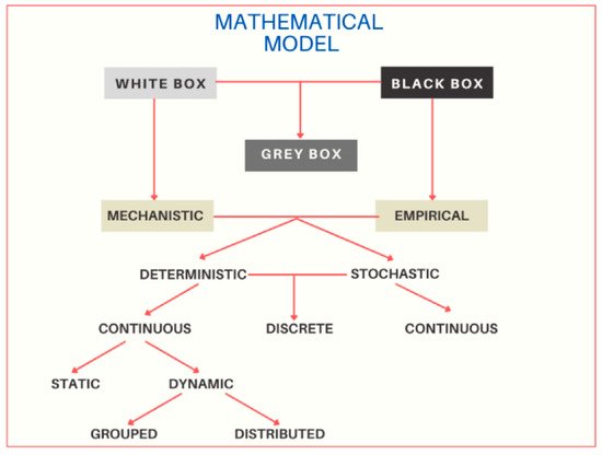
Figure 1. Classification of mathematical models. The diagram shows the three main classifications of the white box, black box and gray box models, and their sub-classifications of the white box or mechanistic, and black box or empirical models. Mechanistic and empirical models can be deterministic or stochastic; and in turn, they can be continuous or discrete.
Empirical models, also called black box models, mainly described a system’s responses by using mathematical or statistical equations without any scientific content, restrictions, or scientific principle. Depending on particular goals, this may be the best type of model to build [44]. Its construction is based only on experimental data and does not explain dynamic mechanisms; this refers to the fact that the system’s process is unknown [40]. Estimating an unknown function from the observations of its values is a problem. The basic advice in this aspect is to estimate models of different complexity and evaluate them using validation data. A good way to restrict certain classes of models’ flexibility is to use a regularized fit criterion. A key issue is finding a sufficiently flexible parameterization model. Another key is to find a suitable “close approach “to the model structure [45]. Researchers usually employ methods for predicting physiological parameters by using intelligent algorithms, such as Support Vector Machines (SVM), Back-Propagation Neural Network (BPNN), Artificial Neural Network (ANN), Deep Neural Network (DNN), and the combination of Wide and Deep Neural Network (WDNN) [46].
Mechanistic models, also called white box models, provide a degree of understanding or explanation of the modeled phenomena. The term “understanding” implies a causal relationship between quantities and mechanisms (processes). A well-built mechanistic model is transparent and open to modifications and extensions, more or less without limits. A mechanistic model is based on people's ideas about how the system works, the important elements, and how they are related [44]. These models allow knowing the input or output variables and the variables involved during the modeling process [40][47]. Mechanistic models are more research-oriented than application-oriented, although this is changing as people's mechanistic models become more reliable. Evaluation of such models is essential, although it is often, and inevitably, rather subjective. Conventional mechanistic models are complex, and unfriendly [44].
Figure 1 shows that both mechanistic and empirical models can be deterministic or stochastic. Determinists make definite quantitative predictions (plant dry-matter or animal intake) without any associated probability distribution. This can be acceptable in many cases; however, it may not be satisfactory for quite changeful quantities or processes (e.g., rain or the migration of diseases, pests, or predators). On the other hand, stochastic models include a random element as a part of the model so that the predictions have a distribution. One problem with stochastic models is that they can be technically difficult to build and complex to test or falsify [44].
In turn, the deterministic and stochastic models can be continuous or discrete. A mathematical model that describes the relationship between continuous signals in time is called time-continuous. Differential equations are frequently used to describe such relationships. A model that directly relates the values of the signals at the sampling times is called a discrete or sampled time model. Such a model is typically described by differential equations [48].
The continuous models are classified as dynamic since they predict how quantities vary with time, so a dynamic model is generally presented as a set of ordinary differential equations with time (t), the independent variable. On the other hand, the continuous models can also be static; they do not contain time as a variable and do not make time-dependent predictions [44].
Finally, dynamic models can be grouped or distributed. Partial differential equations mathematically describe many physical phenomena. The events in the system are, so to speak, scattered over the spatial variables. This description is called the distributed parameter model. If a finite number of changing variables describes the events, it speaks of grouped models. These models are usually expressed by ordinary differential equations [48].
An intermediate model is classified as the semi-empirical or semi-mechanistic model between the black box and white box models. These models are also called gray box or hybrid models; they consist of a combination of empirical and mechanistic models [40].
The practical use of a mathematical model classification lies in understanding “where you are” in the mathematical model space and what types of models might apply to the problem. To understand the nature of mathematical models, they can be defined by the chronological order in which the model’s constituents usually appear. Usually, a system is given first, then there is a question regarding that system, and only then is a mathematical model developed. This process is denoted as SQM, where S is a system, Q is a question relative to S, and M is a set of mathematical states M = (σ1, σ2, …, Σn) which can be used to answer Q. Based on this definition, it is natural to classify mathematical models in an SQM space [36]. Figure 2 shows an approach to visualize this SQM space of mathematical models based on the white box and black box models classification. At the black box, at the beginning of the spectrum, models can perform reliable predictions based on data. At the white box end of the spectrum, mathematical models can be applied to the design, testing, and optimization of computer processes before they are physically carried out. On each of the S, Q, and M axes in Figure 2b, the mathematical models are classified based on a series of criteria compiled from various classification attempts in the literature [36].
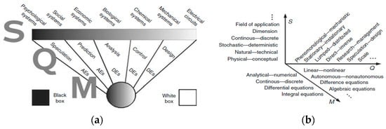
Figure 2. The three dimensions of an SQM mathematical model, where the (S) systems are ranked at the top of the bar; immediately below the bar, there is a list of objectives that the mathematical models in each of the segments can have (which is Q); at the lower end are the corresponding mathematical structures (M) ranging from algebraic equations (Aes) to differential equations (Des). (a) Classification of mathematical models between black and white box models. (b) Classification of mathematical models in the SQM space.
There are different mathematical models related to biochemical, physical, and agroecological variables that estimate photosynthesis at the leaf, plant, or group of plant levels. Therefore, the study of mathematical modeling focused on the photosynthetic process becomes important in the agricultural sector. Since it is a direct indicator of a plant’s health. It also makes it possible to assess the consequences of global climate change on crop growth, since the high concentration of CO2, the increase in temperature and altered rainfall patterns can have serious effects on crop production in the near future [44].
However, to the best of the authors’ knowledge, a study on the diversity of mathematical modeling in the field of scientific research has not been approached nor focused on: the mathematical formulation, the complexity of the model, the validation, the type of crop (at the leaf, plant or canopy level), the analysis of the diversity of variables used with their respective units, as well as the invasiveness in their measurements. Hence, this manuscript presents a selective review of mathematical modeling to estimate photosynthesis.
In the literature, there is a review of the mathematical modeling of photosynthesis developed by Susanne Von Caemmerer. However, here only several models derived from the C3 model by Farquhar, von Caemmerer, and Berry are discussed and compared. The models described and reviewed here describe the assimilation rates of CO2 in a steady state and provide a set of hypotheses collected in a quantitative way that can be used as research tools to interpret experiments both in the field and in the laboratory. Additionally, it also provides tools for reflective experiments [49]. Conversely, above content provides a new vision of the state of the art in mathematical models with certain specifications. This information can be used to develop new mathematical models to estimate photosynthesis with new variables related to the plant’s habitat and with greater relevance to be implemented in electronic systems during the development of photosynthesis estimation equipment.
References
- Marín, M.A. Control Climático y Ciclo de Cultivo. Horticultura 2001, 152, 28–34.
- Stirbet, A.; Lazár, D.; Guo, Y.; Govindjee, G. Photosynthesis: Basics, History and Modelling. Ann. Bot. 2020, 126, 511–537.
- Daniell, H.; Lin, C.-S.; Yu, M.; Chang, W.-J. Chloroplast Genomes: Diversity, Evolution, and Applications in Genetic Engineering. Genome Biol. 2016, 17, 134.
- Blankenship, R.E. Molecular Mechanisms of Photosynthesis; John Wiley & Sons: New York, NY, USA, 2021.
- Maxwell, K.; Johnson, G.N. Chlorophyll Fluorescence—A Practical Guide. J. Exp. Bot. 2000, 51, 659–668.
- Tillery, B.; Enger, E.; Ross, F. Integratsssed Science; Higher Education; McGraw-Hill: New York, NY, USA, 2012.
- Shipman, J.; Wilson, J.D.; Higgins, C.A.; Lou, B. An Introduction to Physical Science; Cengage Learning: Boston, MA, USA, 2020.
- Azcon-Bieto, J.; Talón, M. Fundamentos de Fisiología Vegetal; McGraw-Hill: Interamericana de España, Barcelona, Spain, 2000.
- Cheng, Y.; He, D. A Photosynthesis Continuous Monitoring System for CAM Plants. Int. J. Agric. Biol. Eng. 2019, 12, 141–146.
- West-Eberhard, M.J.; Smith, J.A.C.; Winter, K. Photosynthesis, Reorganized. Science 2011, 332, 311–312.
- Fereres Castiel, E.; Martín, V.; Francisco, J. Fitotecnia: Principios de Agronomía para Una Agricultura Sostenible; Mundi-Prensa Libros: Madrid, Spain, 2017.
- Taiz, L.; Zeiger, E.; Møller, I.M.; Murphy, A. Plant Physiology and Development; Sinauer Associates Incorporated: Sunderland, MA, USA, 2015.
- Climático, C.; Biodiversidad, Y. Documento Técnico V Del IPCC; IPCC: Geneva, Switzerland, 2002.
- Bidwell, R.G.S. Fisiología Vegetal; AGT: Mexico City, Mexico, 1993.
- Murchie, E.H.; Pinto, M.; Horton, P. Agriculture and the New Challenges for Photosynthesis Research. New Phytol. 2009, 181, 532–552.
- Zhang, Y.; Xiao, X.; Wu, X.; Zhou, S.; Zhang, G.; Qin, Y.; Dong, J. A Global Moderate Resolution Dataset of Gross Primary Production of Vegetation for 2000–2016. Sci. Data 2017, 4, 170165.
- Ryu, Y.; Berry, J.A.; Baldocchi, D.D. What Is Global Photosynthesis? History, Uncertainties and Opportunities. Remote Sens. Environ. 2019, 223, 95–114.
- Wu, A.; Hammer, G.L.; Doherty, A.; von Caemmerer, S.; Farquhar, G.D. Quantifying Impacts of Enhancing Photosynthesis on Crop Yield. Nat. Plants 2019, 5, 380–388.
- Morales, F.; Ancín, M.; Fakhet, D.; González-Torralba, J.; Gámez, A.L.; Seminario, A.; Soba, D.; Ben Mariem, S.; Garriga, M.; Aranjuelo, I. Photosynthetic Metabolism under Stressful Growth Conditions as a Bases for Crop Breeding and Yield Improvement. Plants 2020, 9, 88.
- Sinclair, T.R.; Rufty, T.W.; Lewis, R.S. Increasing Photosynthesis: Unlikely Solution for World Food Problem. Trends Plant Sci. 2019, 24, 1032–1039.
- Shevela, D.; Bjorn, L.O. Photosynthesis: Solar Energy for Life; World Scientific Publishing: Singapore, 2018.
- Tenhunen, J.D.; Weber, J.A.; Yocum, C.S.; Gates, D.M. Development of a Photosynthesis Model with an Emphasis on Ecological Applications. Oecologia 1976, 26, 101–119.
- Field, C.B.; Ball, J.T.; Berry, J.A. Photosynthesis: Principles and Field Techniques. In Plant Physiological Ecology; Springer: New York, NY, USA, 2000; pp. 209–253.
- Wolfbeis, O.S. Materials for Fluorescence-Based Optical Chemical Sensors. J. Mater. Chem. 2005, 15, 2657–2669.
- Millan-Almaraz, J.R.; Guevara-Gonzalez, R.G.; Troncoso, R.R.-; Osornio-Rios, R.A.; Torres-Pacheco, I. Advantages and Disadvantages on Photosynthesis Measurement Techniques: A Review. Afr. J. Biotechnol. 2009, 8, 7340–7349.
- Busch, F.A. Photosynthetic Gas Exchange in Land Plants at the Leaf Level. In Photosynthesis; Springer: New York, NY, USA, 2018; pp. 25–44.
- Walker, B.J.; Busch, F.A.; Driever, S.M.; Kromdijk, J.; Lawson, T. Survey of Tools for Measuring In Vivo Photosynthesis. Photosynthesis 2018, 1770, 3–24.
- Bassow, S.L.; Bazzaz, F.A. How Environmental Conditions Affect Canopy Leaf-Level Photosynthesis in Four Deciduous Tree Species. Ecology 1998, 79, 2660–2675.
- Schulze, E.-D. A New Type of Climatized Gas Exchange Chamber for Net Photosynthesis and Transpiration Measurements in the Field. Oecologia 1972, 10, 243–251.
- Hunt, S. Measurements of Photosynthesis and Respiration in Plants. Physiol. Plant. 2003, 117, 314–325.
- Takahashi, M.; Ishiji, T.; Kawashima, N. Handmade Oxygen and Carbon Dioxide Sensors for Monitoring the Photosynthesis Process as Instruction Material for Science Education. Sens. Actuators B Chem. 2001, 77, 237–243.
- Biosciences LI-6400XT System. Photosyntesis, Fluorescence, Respiration. 2014. Available online: https://www.licor.com/env/products/photosynthesis/LI-6400XT/ (accessed on 28 March 2022).
- Kawachi, N.; Sakamoto, K.; Ishii, S.; Fujimaki, S.; Suzui, N.; Ishioka, N.S.; Matsuhashi, S. Kinetic Analysis of Carbon-11-Labeled Carbon Dioxide for Studying Photosynthesis in a Leaf Using Positron Emitting Tracer Imaging System. IEEE Trans. Nucl. Sci. 2006, 53, 2991–2997.
- Taiz, L. Plant Physiology, 5th ed.; Sinauer Associates Inc.: Sunderland, MA, USA, 2006.
- Hermand, J.-P. Photosynthesis of Seagrasses Observed in Situ from Acoustic Measurements. In Proceedings of the Oceans’ 04 MTS/IEEE Techno-Ocean’04 (IEEE Cat. No. 04CH37600), Kobe, Japan, 9–12 November 2004; Volume 1, pp. 433–437.
- Velten, K. Mathematical Modeling and Simulation: Introduction for Scientists and Engineers; John Wiley & Sons: New York, NY, USA, 2009.
- Hesketh, J.D. Predicting Photosynthesis for Ecosystem Models: Volume II; CRC Press: Boca Raton, FL, USA, 2017; ISBN 978-1-351-07595-4.
- Zufferey, V.; Murisier, F.; Schultz, H.R. A Model Analysis of the Photosynthetic Response of Vitis vinifera L. Cvs Riesling and Chasselas Leaves in the Field: I. Interaction of Age, Light and Temperature. VITIS 2000, 39, 19–26.
- Polerecky, L.; Lott, C.; Weber, M. In Situ Measurement of Gross Photosynthesis Using a Microsensor-Based Light-Shade Shift Method. Limnol. Oceanogr. Methods 2008, 6, 373–383.
- Torres-Pacheco, I.; Padilla-Medina, J.A.; Osornio-Rios, R.A.; de Jesus Romero-Troncoso, R.; Villasentilde, C.; Rico-Garcia, E.; Guevara-Gonzalez, R.G. Description of Photosynthesis Measurement Methods in Green Plants Involving Optical Techniques, Advantages and Limitations. Afr. J. Agric. Res. 2011, 6, 2638–2647.
- Magney, T.S.; Frankenberg, C.; Fisher, J.B.; Sun, Y.; North, G.B.; Davis, T.S.; Kornfeld, A.; Siebke, K. Connecting Active to Passive Fluorescence with Photosynthesis: A Method for Evaluating Remote Sensing Measurements of Chl Fluorescence. New Phytol. 2017, 215, 1594–1608.
- Aziz, H.A.; Dianursanti, D. Production of Microalgae Nannochloropsis oculata Biomass in a Bubble Column Photobioreactor with Integrated Lighting through Adjustment of Light Intensity and Air Flow Rate. AIP Conf. Proc. 2018, 2024, 020040.
- Kitić, G.; Tagarakis, A.; Cselyuszka, N.; Panić, M.; Birgermajer, S.; Sakulski, D.; Matović, J. A New Low-Cost Portable Multispectral Optical Device for Precise Plant Status Assessment. Comput. Electron. Agric. 2019, 162, 300–308.
- Thornley, J.H.M.; France, J. Mathematical Models in Agriculture: Quantitative Methods for the Plant, Animal and Ecological Sciences; CABI: Wallingford, UK, 2007; ISBN 978-0-85199-010-1.
- Ljung, L. Black-Box Models from Input-Output Measurements. In Proceedings of the IMTC 2001. In Proceedings of the 18th IEEE Instrumentation and Measurement Technology Conference. Rediscovering Measurement in the Age of Informatics (Cat. No.01CH 37188), Budapest, Hungary, 21–23 May 2001; Volume 1, pp. 138–146.
- Hu, P.; Sun, Y.; Zhang, Y.; Dong, J.; Zhang, X. Application of WDNN for Photosynthetic Rate Prediction in Greenhouse. In Proceedings of the IEEE 2nd International Conference on Big Data, Artificial Intelligence and Internet of Things Engineering (ICBAIE), Nanchang, China, 26–28 March 2021; pp. 331–336.
- Guidotti, R.; Monreale, A.; Ruggieri, S.; Turini, F.; Giannotti, F.; Pedreschi, D. A Survey of Methods for Explaining Black Box Models. ACM Comput. Surv. 2018, 51, 93.
- Ljung, L.; Glad, T. Modeling of Dynamic Systems; PTR Ptrnyice-Hall: Hoboken, NJ, USA, 1994.
- Von Caemmerer, S. Steady-State Models of Photosynthesis. Plant Cell Environ. 2013, 36, 1617–1630.
More
Information
Subjects:
Mathematics, Applied
Contributors
MDPI registered users' name will be linked to their SciProfiles pages. To register with us, please refer to https://encyclopedia.pub/register
:
View Times:
2.3K
Entry Collection:
Environmental Sciences
Revisions:
3 times
(View History)
Update Date:
22 Jun 2022
Table of Contents


Notice
You are not a member of the advisory board for this topic. If you want to update advisory board member profile, please contact office@encyclopedia.pub.
OK
Confirm
Only members of the Encyclopedia advisory board for this topic are allowed to note entries. Would you like to become an advisory board member of the Encyclopedia?
Yes
No
${ textCharacter }/${ maxCharacter }
Submit
Cancel
Back
Comments
${ item }
|
${ item.createdUser.fullName }
${ item.createdAt }
${ item.vote }
${ item.reply }
Delete
${ reply.createdUser.fullName }
${ reply.createdAt }
${ reply.vote }
Delete
There is no reply to this comment~
${ item.replyTextCharacter }/${ item.replyMaxCharacter }
Submit
Cancel
More
No more~
There is no comment~
${ textCharacter }/${ maxCharacter }
Submit
Cancel
${ selectedItem.replyTextCharacter }/${ selectedItem.replyMaxCharacter }
Submit
Cancel
Confirm
Are you sure to Delete?
Yes
No