Your browser does not fully support modern features. Please upgrade for a smoother experience.
Please note this is a comparison between Version 1 by Luz del Carmen García Rodríguez and Version 3 by Conner Chen.
Photosynthesis is a process that indicates the productivity of crops. The estimation of this variable can be achieved through methods based on mathematical models.
- net photosynthesis
- photosynthetic rate
- mathematical models
1. Photosynthesis Process
Plants perform physiological functions that allow them to grow, develop, and reproduce. For their development and growth, plants require energy from sunlight, assimilated carbon dioxide (CO2), hydrogen, mineral nutrients, oxygen (O2), and a suitable temperature both in air and roots [1][2][1,2]. A fundamental physiological process for the vegetable kingdom is photosynthesis. The photosynthesis process occurs in terrestrial and aquatic plants, algae, and some types of bacteria that are essential for living species [3]. Photosynthesis is a process by which plants convert light energy into chemical energy to obtain sugar as a final product. On the other hand, another photosynthetic reaction is oxygenic, which is released into the atmosphere as a waste, being useful for the biological process of respiration [4].
Chloroplasts (plant organelles located in the leaf) are active metabolic centers that capture solar energy through chlorophyll (green pigment) and manufacture carbohydrates (glucose molecules) through the process of photosynthesis [3]. The energy from light absorbed by chlorophyll molecules in a leaf can take one of three ways: it can be used to drive photosynthesis; excess energy can be dissipated as heat, or it can be re-emitted as light-chlorophyll fluorescence [5]. Glucose is one of the main molecules that serve as an energy source for plants and animals. It is found in plant sap and in the human bloodstream, where it is known as “blood sugar” [6][7][6,7]. Then, through photosynthesis, plants produce glucose for their food and dispose of valuable oxygen for the respiration of other living beings. Plants can capture carbon dioxide and release oxygen during the day, but they undergo another change at night: they absorb oxygen and release carbon dioxide [8].
Photosynthesis is divided into two phases: In the first phase, absorption and conversion of energy happen; while in the second, the intake and assimilation of carbon occur. Light energy is absorbed by photosensitive biomolecules and transformed into a stable biochemical energy form. The constituent elements are taken from inorganic mineral sources (water, H2O; carbon dioxide, CO2; nitrates, NO−3; sulfates, SO2−4, among others.) and are incorporated into metabolizable organic biomolecules. Both phases are perfectly coordinated and interrelated. Traditionally, these phases have been called the light phase and the light-independent phase. The first phase is produced only by utilizing sunlight, which will provide us with oxygen, ATP (adenosine triphosphate), and NADPH (nicotinamide adenine dinucleotide phosphate). In the second phase (it can occur during the day and also at night), the Calvin cycle is carried out where glucose is produced by using the ATP, NADPH, and CO2 generated in the light phase [2][8][2,8].
The essential and predominant element in organic material is carbon. In photosynthesis, carbon is taken from the air’s carbon dioxide (CO2). Generally, in terrestrial plants, CO2 is incorporated from the atmosphere through stomata. Algae and aquatic plants take it from the CO2 dissolved in the surrounding water. At night, when photosynthesis is not active and, therefore, there is no demand for CO2 inside the leaf, the stomatal openings are reduced preventing unnecessary water loss. In the morning, when the water supply is abundant and solar radiation favors photosynthetic activity, the demand for CO2 inside the leaf is big and the stomatal pores are wide open, reducing the stomatal resistance to the diffusion of the CO2 [8].
Plants have developed three photosynthetic systems, C3, C4, and CAM (Crassulacean acid metabolism), with different anatomical and chemical characteristics [9], the C3 type being the most common [10][11][10,11]. The main difference between the types of photosynthesis lies in the way CO2 is synthesized. The first step in the Calvin cycle is carbon dioxide fixation by rubisco. Plants that use only this “standard” carbon fixation mechanism are called C3 plants because of the three-carbon compound (3-PGA) that they produce during this part of the photosynthetic process. In C4 plants, the light-dependent reactions and the Calvin cycle are physically separated: the light-dependent reactions occur in the cells of the mesophyll (spongy tissue in the center of the leaf) and the Calvin cycle occurs in special cells around the veins of the leaf. These cells are called vascular bundle cells. Some plants adapted to dry environments use the crassulaceae acid metabolism (CAM) pathway to minimize photorespiration. Instead of separating the light-dependent reactions and the use of CO2 in the Calvin cycle, the temporary separation of photosynthetic processes in CAM plants causes carbon assimilation to take place at night. At night, they open their stomata so that the CO2 diffuses into the leaves. This CO2 is fixed to oxaloacetate by PEP carboxylase (the same step that C4 plants use), which is then converted into malate or another organic acid [8]. The organic acid is stored inside vacuoles until the next day. During the day, CAM plants do not open their stomata, but they can still carry out photosynthesis. Because organic acids are transported out of vacuoles and broken down to release CO2, which enters the Calvin cycle. This controlled cycle maintains a high concentration of CO2 around rubisco [4]. The ability to represent the three photosynthetic types (C3, C4, and CAM) has important implications for studying natural ecosystems and agroecosystems [12].
The described complex process of photosynthesis must work, integrally and efficiently, in an environment where there is an enormous natural variability of factors that affect the rate of photosynthesis. For instance, light, environment temperature, air humidity, availability of water, and mineral nutrients in the soil, among others. Carbon dioxide (CO2) can also be considered as part of this list of relevant factors due to global climate change [13]. The photosynthesis rate of a leaf is conditioned by one of more than 50 individual reactions, each presenting its response to each environmental variable. This photosynthetic rate can widely vary between days and also throughout seasons, due to environmental factors such as light and temperature. It can also vary in the longer term during the coming decades as a response to increasing atmospheric CO2 levels. The increase in CO2 and other greenhouse gases in the atmosphere can cause global climate change. As can be understood, each of the aforementioned environmental factors affects the photosynthesis rate in a different way, depending on the time scale [8].
Photosynthesis is important for many reasons. From humanity’s point of view, it produces food and oxygen; therefore, it is often studied in its end products. However, these are secondary aspects of an integral process. The most important aspects are capturing and transforming light [14]. A critical component of crop production is the ability to produce more biomass [15].
Photosynthesis at the ecosystem scale, also known as the gross primary productivity (GPP), is the first step of CO2 entering the biosphere from the atmosphere. Over the past century, with the increasing carbon release from landcover change and fossil fuel burning, the CO2 accumulation rate on land, in the ocean and in the atmosphere has continuously increased. The increment of CO2 in Earth’s atmosphere is the major cause of global climate change. A major contribution to this high variability comes from GPP, as the photosynthesis process is vulnerable to droughts, heatwaves, floods, frost, and other types of disturbances. An accurate estimation of GPP will not only provide information about the ecosystem response to these extreme events but also help to predict the future carbon cycle dynamics [16].
For the agronomic sector the research about photosynthesis is useful in many aspects, such as: determining the state of crops or of certain plants; indicating crop production; helping in crop-health control; helping with the optimization of natural resources; detecting genetic alterations in plants to know how plants react to stressful situations; and serving as a predictive indicator of biomass accumulation in green plants [17][18][19][20][21][22][17,18,19,20,21,22].
2. Methods for Inferring Photosynthesis
Many of the methods for inferring photosynthesis are invasive; they physically or chemically interfere with the plant, altering its natural process during measurement. Non-invasive methods do not alter the plant’s natural process since there is no contact with the specimen [23][24][23,24]. Millan et al. [25] presented a review of the advantages and disadvantages of the methods used for photosynthesis estimation. Table 1 shows the classification of these methods. CO2 exchange is the most used method for constructing commercial and experimental equipment [26][27][26,27]. It is possible to measure photosynthesis at the level of individual leaves, whole plants, plant canopies, and even forests [28][29][28,29].Table 1.
Classification of the methods used for photosynthesis estimation and their general description.
| Methods Used for Photosynthesis Estimation | Description |
|---|---|
| Destructive | Involves cutting a whole plant or only a portion of it to estimate the photosynthetic activity based on the accumulation of dry matter in the plant, from the point of germination until it is cut [25]. |
| Manometric | Consists of direct measurement of oxygen (O2) pressure or carbon dioxide (CO2) in an isolated chamber with photosynthetic organisms [30]. |
| Electrochemical | Uses electrochemical electrodes to measure O2, CO2, or pH in aqueous solutions of the sample to detect variations that depend on photosynthetic activity [30]. |
| Gas exchange | Consists of isolating the sample for analysis in a closed chamber to quantify the CO2 concentration [29][31][29,31]. Concentrated CO2 gas is detected by an infrared gas sensor (called IRGA for Infra-Red Gas Analysis sensors) [32] |
| Carbon isotopes | Uses carbon isotopes such as 11C, 12C, and 14C to produce incorporated CO2 with radioactivity. This methodology is applied to analyze samples in isolated and illuminated chambers to produce a maximum fixation of radioactive CO2 during photosynthesis [33][34][33,34]. The main disadvantage is that it is destructive as it fixes a radioactive compound onto the sample; and its precision depends on lighting conditions. |
| Acoustic waves | Based on the principle of sound wave distortion in the medium in which waves propagate. The technique involves placing an acoustic transmitter on the seabed area where you want to monitor photosynthetic activity. The disadvantage is that it dependent on water conditions and sensitive to environmental disturbances [35]. |
| Fluorescence | Way in which a certain amount of light energy absorbed by chlorophylls is dissipated. The fluorescence emission can be analyzed and quantified, which provides information on the electron transport rate, the quantum yield and the existence of photoinhibition of photosynthesis. Indeed, fluorescence is used in various ways, and it has different applications. The interested reader is referred to reference [5][8][24][5,8,24]. |
| Mathematical modeling | Equation or a set of equations that represent a system’s behavior. There is a correspondence between the model variables and the observable quantities [36]. |
3. Mathematical Modeling
Any branch of science, as it progresses from qualitative to quantitative, is likely to reach the point where the use of mathematics to connect experiment and theory is essential. Mathematical modeling consists of the following steps [44]:- Definitions;
- Systems analysis;
- Modeling;
- Simulation;
- Validation.
-
Definitions;
-
Systems analysis;
-
Modeling;
-
Simulation;
-
Validation.
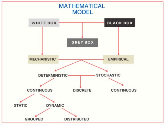
Figure 1. Classification of mathematical models. The diagram shows the three main classifications of the white box, black box and gray box models, and their sub-classifications of the white box or mechanistic, and black box or empirical models. Mechanistic and empirical models can be deterministic or stochastic; and in turn, they can be continuous or discrete.
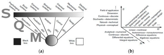
Figure 2. The three dimensions of an SQM mathematical model, where the (S) systems are ranked at the top of the bar; immediately below the bar, there is a list of objectives that the mathematical models in each of the segments can have (which is Q); at the lower end are the corresponding mathematical structures (M) ranging from algebraic equations (Aes) to differential equations (Des). (a) Classification of mathematical models between black and white box models. (b) Classification of mathematical models in the SQM space. Modified from [36].