Your browser does not fully support modern features. Please upgrade for a smoother experience.
Submitted Successfully!
 +1 credit
Thank you for your contribution! You can also upload a video entry or images related to this topic.
For video creation, please contact our Academic Video Service.
| Version | Summary | Created by | Modification | Content Size | Created at | Operation |
|---|---|---|---|---|---|---|
| 1 | Yuyang LIU | -- | 3456 | 2022-06-15 11:52:36 | | | |
| 2 | Peter Tang | Meta information modification | 3456 | 2022-06-15 12:26:35 | | |
Video Upload Options
We provide professional Academic Video Service to translate complex research into visually appealing presentations. Would you like to try it?
Cite
If you have any further questions, please contact Encyclopedia Editorial Office.
Liu, Y.; Zhang, X.; Guo, W.; Kang, L.; , .; Yu, R.; Sun, Y.; Pan, M. 3D Geological Property Modeling Methods. Encyclopedia. Available online: https://encyclopedia.pub/entry/24059 (accessed on 12 June 2026).
Liu Y, Zhang X, Guo W, Kang L, , Yu R, et al. 3D Geological Property Modeling Methods. Encyclopedia. Available at: https://encyclopedia.pub/entry/24059. Accessed June 12, 2026.
Liu, Yuyang, Xiaowei Zhang, Wei Guo, Lixia Kang, , Rongze Yu, Yunping Sun, Mao Pan. "3D Geological Property Modeling Methods" Encyclopedia, https://encyclopedia.pub/entry/24059 (accessed June 12, 2026).
Liu, Y., Zhang, X., Guo, W., Kang, L., , ., Yu, R., Sun, Y., & Pan, M. (2022, June 15). 3D Geological Property Modeling Methods. In Encyclopedia. https://encyclopedia.pub/entry/24059
Liu, Yuyang, et al. "3D Geological Property Modeling Methods." Encyclopedia. Web. 15 June, 2022.
Copy Citation
Three-dimensional (3D) geological property modeling is used to quantitatively characterize various geological attributes in 3D space based on geostatistics with the help of computer visualization technology, and the results are often stored in grid data. The 3D geological property modeling includes two main components, grid model generation and property interpolation.
3D model
property modeling
grid generation
property interpolation
geostatistics
1. Introduction
Three-dimensional (3D) geological property modeling refers to the quantitative characterization of various geological features in 3D space in digital form based on geostatistics using computer visualization technology. It serves as the basis for evaluating mineral resource assessments, reservoir physical property simulations, and reservoir numerical simulations [1][2].
The main application of 3D property modeling in the petroleum field is to establish a geological model of the reservoir; this type of modeling is therefore also called reservoir modeling. The characterization of 3D reservoir models provides an in-depth understanding of the macroscopic distribution, internal structure, physical parameters, and variation characteristics of oil and gas reservoirs, and this understanding is of great importance for oil and gas exploration and development [3]. Geostatistics, which is the core method of 3D property modeling, was proposed by Journel in the 1970s for application in petroleum exploration and development [4][5] and has been widely used and developed since then. The advantage of geostatistics is its ability to integrate data according to the source and reliability of the data and to integrate various information, such as core, log, and seismic data, into the model while ensuring data consistency. In addition, geostatistics can also provide uncertainty assessment as a basis for risk evaluation. In China, research on the theory, methods, and applications of geostatistics started around the 1980s [6], and the application of geostatistics in reservoir descriptions for reservoir geological modeling began in the early 1990s. Since Qiu [7] introduced the related work on reservoir modeling, Zhang and Wang [8], Yu and Li [9], and Zhang et al. [10] successively carried out research on reservoir modeling methods for actual reservoirs in China; this research laid the foundation for applying reservoir modeling technology in oilfield development. Since then, with the development of computer technology and the research of numerous studies in petroleum science and technology, the methods and techniques of reservoir modeling and its application to various reservoir types have developed rapidly.
The oil and gas reservoirs in China are mainly terrestrial oil reservoirs with very complex subsurface conditions; consequently, establishing a 3D property model for reservoir characterization is difficult. At present, most oilfields have entered the middle and late stages of development and are in a state of high water content. The balance between injection and production poses an increasingly prominent problem, so it is especially important to determine the amount and distribution of the remaining oil in the reservoir. In addition, today’s petroleum exploration and development focus on unconventional oil and gas reservoirs, such as shale gas and tight sandstone gas. Although such oil and gas reservoirs are abundant in China, they are characterized by low porosity, low permeability, and high water saturation. Therefore, compared with that of conventional oil and gas reservoirs, the development of unconventional oil and gas reservoirs is bound to pose new requirements for reservoir modeling. To solve these problems, there is an urgent need to establish a more refined reservoir model. Therefore, it is necessary to study grid framework models and geostatistical theories and methods in depth so that they can accurately characterize the reservoir at various levels and describe the heterogeneity of the reservoir while quantitatively evaluating the uncertainty of the model and reducing the risk of exploration and development. Therefore, studying 3D property modeling methods can provide a powerful tool for improving the recovery of oil reservoirs in China and offer theoretical guidance for effectively recovering the remaining oil and developing unconventional oil and gas reservoirs.
3D property modeling represents the heterogeneity of properties in the geological body, thereby reflecting the distribution of the characteristic values of a certain class of physical and chemical properties of the geological body in 3D space, and the results are stored in raster data [11][12]. Based on this definition, 3D property modeling includes two main components: 3D grid model generation and property interpolation. In petroleum exploration and development, the 3D raster model is also referred to as the reservoir grid, and due to the complexity of the physical structure of the reservoir, geostatistics are applied to the model’s property interpolation.
2. Research on Reservoir Grid Generation Method
Building a 3D reservoir grid model is a key intermediate process and importantly affects the subsequent reservoir property modeling and numerical simulation based on geostatistics. In modeling a reservoir by using geostatistical tools, the gridding process essentially determines how to characterize the macroscopic homogeneity of the reservoir. Since geostatistics are implemented on logical grids, a grid with excessive and excessively large distortion can easily cause the variogram to become distorted, thus affecting the accuracy and reliability of the modeling of properties, such as sedimentary facies and pore permeability [13][14]. Additionally, the shape and resolution of the grid affect the accuracy and speed of the numerical simulation of the reservoir [14][15].
Research on reservoir grid models has been carried out for many years, resulting in many grid types. Zakrevsky [16] conducted comprehensive gridding and outlined the general procedure of grid generation. Reservoir grids are categorized mainly into structured grids and unstructured grids. Structured grids are typically generated using hexahedra and are organized in an orderly manner with i, j, and k, such as Cartesian grids and corner point grids, while unstructured grids include tetrahedral grids and perpendicular bisector (PEBI) grids. In stratified deposits such as oil sand, often, the Cartesian grid is transformed to a stratigraphic grid using a non-linear coordinate transformation, which is referred to as unfolding. Thom [17] compared the characteristics of the s-grid, faulted s-grid, and pillar grid as well as these grids’ performance differences in property distribution, grid coarsening, and numerical simulation. As show in Figure 1, For the s-grid, faulted s-grid, and pillar grid, the main difference is that they contain different fault treatment approaches. Three different examples are extracted in Figure 1a–c, and the conceptual models are drawn, as show in Figure 1d, to show the different fault treatment approaches. S-grid is also known as stair-step grid; the sides of this kind of grid cell remain vertical and are controlled by an orthogonal footprint [17], as show in Figure 1a. Faulted s-grid is known as Jewel Grid; the grid cells are split exactly at the local position of the fault plane, as show in Figure 1b [17]. Pillar grid is widely used in petroleum engineering, and the most common grid is the corner point grid. For the position of faults, the pillar that controls the grid cells is parallel with the fault lines. Thus, the fault should be simplified when the fault is too complicated, as shown in Figure 1c.
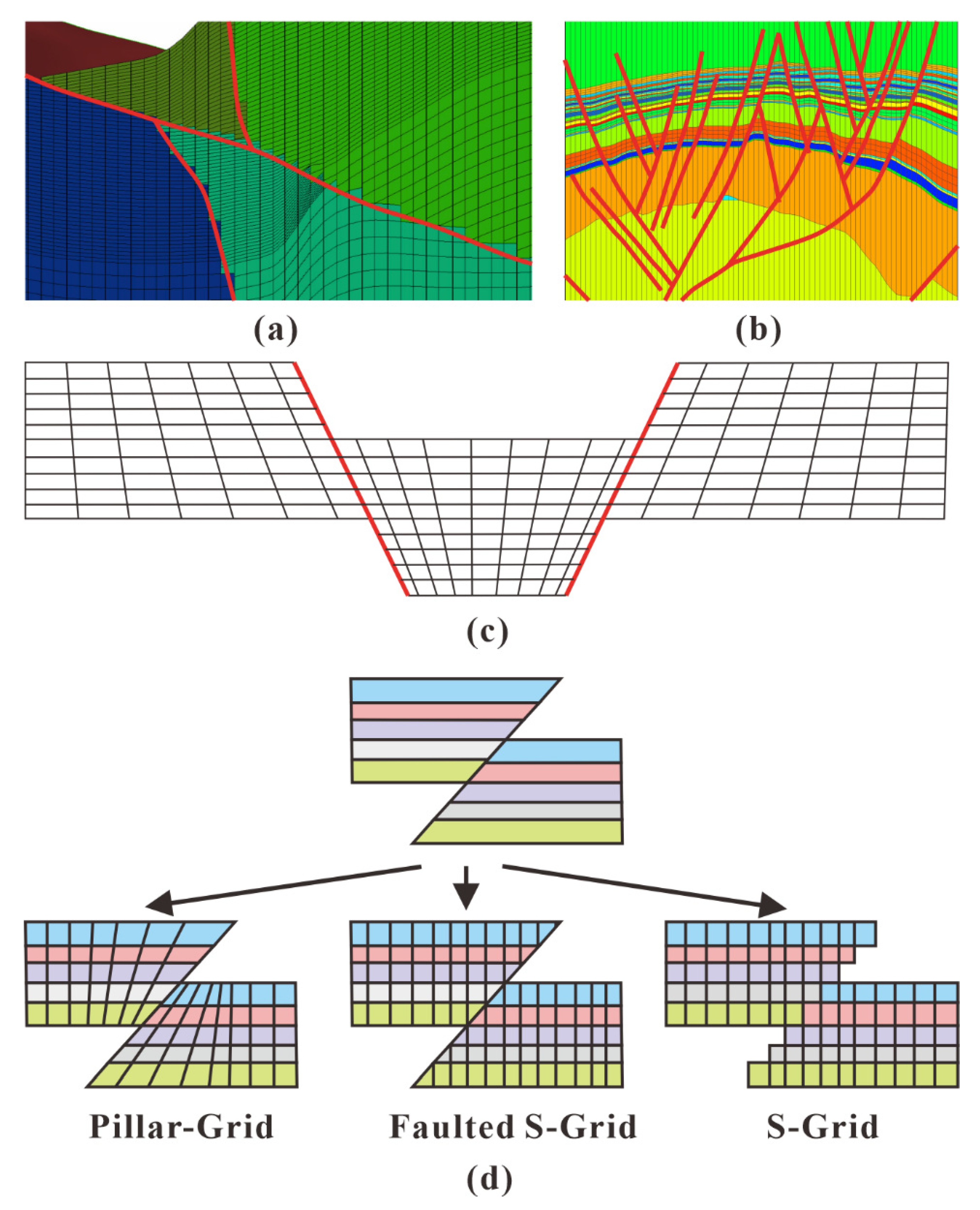
Figure 1. Comparison of s-grid, faulted s-grid, and pillar grid [17]: (a) example of s-grid; (b) example of faulted s-grid; (c) example of pillar grid; (d) theoretical model of s-grid, faulted s-grid, and pillar grid for the processing of faults.
Gringarten et al. and Mallet et al. [18][19] divided the grids into “geological grids” for geostatistical property modeling and “fluid simulation grids” for numerical simulation based on the different needs of reservoir modelers and digital modeling engineers for grid use. In the many grid studies, the corner point grid represented by the pillar grid has been the hotspot of research, with the most mature application. Pillar grid generation involves three main steps [20][21]: (1) a fault model is formed by simulating the fault using pillars; (2) gridding is carried out by combining fault pillars into a 3D grid framework; and (3) vertical stratification is conducted by generating initial layer surfaces on the grid framework for geological stratification. The pillar grid is characterized by its grid orientation along fault lines, boundary lines, or pinch-out lines, indicating that the grid can be distorted, thus overcoming the inflexibility of the orthogonal Cartesian grids and allowing for easy simulations of faults, boundaries, and pinch-outs [22][23]. With the development of technology and the continuous improvement in reservoir simulation accuracy, the defects of the pillar grid are gradually exposed as follows. First, due to the limitation of the geometric location of pillars, it is necessary to simplify the fault when using pillars to construct a complex fault network. Second, on the one hand, the nonorthogonality of the pillar grid makes calculating conductivity during numerical simulation difficult; on the other hand, the nonorthogonality of the pillar grid affects the accuracy of the results. Ruiu [24] proposed a grid generation method that adopts the form of a Cartesian grid at the global level and simulates the fault by truncating the hexahedron, thereby finally constructing an XY-orthogonal and locally truncated grid model. This grid can express the shape of the fault while avoiding the loss of orthogonality due to distortion, but the grid generates many polyhedral grids in models with many faults, thereby also affecting the fluid simulation operations. After analyzing the limitations of the pillar grid, Gringarten [25] proposed a vertical stair-step grid that is more suitable for fluid simulation and experimentally demonstrated that this type of grid outperforms the pillar grid in terms of grid coarsening and fluid simulation; the author did not give the method for generating this grid.
In addition, many studies have been devoted to unstructured grids. The PEBI grid is flexible and locally orthogonal, thus reducing the influence of grid orientation on the results. In 1988, Heinemann et al. [26] proposed the implementation of the PEBI grid based on the Voronoi diagram for the numerical simulation of the reservoir grid and then improved the grid with dynamic refinement as needed [27][28][29]. Palagi of Stanford University [30][31][32] studied the use of the Voronoi grid, which is essentially the PEBI grid, to simulate vertical and horizontal wells and performed numerical simulation of reservoirs. Since then, scholars have successively carried out research on 3D PEBI grids along with investigation and improvement in different application environments [33][34][35][36]. Additionally, many studies on PEBI grids have been published in recent years by Chinese researchers. Xie [37] and Lin et al. [38][39][40] systematically elaborated the application of PEBI grids in the numerical simulation of reservoirs. Liu [41] addressed the problem of fine numerical simulation of reservoirs by adopting an idea of a hybrid grid consisting of a radial grid in the oil well area and a PEBI grid in the reservoir area. Ref. [42] proposed a similar idea on hybrid grids.
Xiang [43] and Zha [44][45][46] studied the generation algorithm of two-dimensional (2D) PEBI grids, but did not fully address the generation algorithm of 3D PEBI grids. In general, the numerical simulation solutions of PEBI grids are not mature enough and not widely used. In addition, the research on PEBI grids is mainly for the numerical simulation of reservoirs; there are few studies on how PEBI grids are generated and maintain geological significance in geological modeling. In other words, other grids generally need to be transformed before PEBI grids can be used for the numerical simulation of reservoirs.
3. Interpolation Methods for 3D Property Modeling
3.1. Traditional Geostatistical Methods
There is often much spatial variability when dealing with subsurface space modeling in Earth science. Proposed by Matheron [47], geostatistics is a tool to quantify this variability to enable geologists to predict behavior and make the most useful decisions under the constraints of limited knowledge and resources. The major techniques for generating a 3D model of the geological variables are the main focus, especially the interpolation methods; thus, the principal component analysis (PCA), maximum autocorrelation factor (MAF), projection pursuit multivariate transform (PPMT), and related methods are not considered. The PCA, MAF, PPMT, and other multivariate transforms methods are commonly used to simulate correlated variables independently without the requirement of fitting a linear model. In addition, these approaches can be applied in the data preparation procedure for the geostatistics approaches dealing with multivariate analysis.
Geological phenomena, especially in the petroleum industry, follow a series of complex physical rules that cannot be expressed by simplified models. Reservoir properties, such as porosity and permeability, are needed in reservoir fluid simulation equations to predict oil production and are required at each spatial location; however, porosity and permeability can be obtained only in sparse wells. In other words, for economic reasons, it is generally impossible to accurately and definitively obtain all the information required for a subsurface model. Therefore, spatial uncertainty is a fundamental concept in Earth science. In the early days of the oil industry, practitioners tended to think deterministically and thus expected to obtain a single estimate of oil production. Today, uncertainty is widely accepted.
Geostatistics captures this spatial uncertainty by generating multiple reasonable property models (also known as stochastic realization). By integrating information from different sources, such as logging, coring, geological interpretation, or seismic data, the study area and the true expression of this uncertainty can be obtained. Matheron [48] introduced the regionalized variable Z(h) as the value of characteristic Z of a geological phenomenon at location u. Regionalization means that variables expand in space and exhibit a specific spatial structure. If this concept is ignored, the variables are randomly distributed in the reference region and thus do not exhibit any spatial continuity. However, physical processes in geology are not random in space and have spatial continuity in their properties. For example, the continuity of the river channel formed by a river flowing down the hillside is controlled by the complex physical phenomena along the path of the river, and the mineral deposits tend to be concentrated in certain specific spaces. Thus, the regionalization of variables is the main principle by which geostatistics differs from statistics. It would be impossible to make predictions if spatial continuity does not exist. However, the physical laws that determine spatial continuity cannot be accurately modeled due to the lack of information. To quantify spatial uncertainty, a mathematical model is needed to describe the spatial structure of the variables in the study area. For example, the spatial trends in the data and the isotropy or anisotropy of the variables can be obtained by defining a spatial variable model in geostatistics.
Geostatistical methods have evolved over the decades into two-point geostatistical methods (including the kriging method, deterministic simulation method, and stochastic simulation methods), object-based methods, and multiple-point geostatistics. The methods differ in how their spatial continuity and uncertainty models are expressed and how direct data (such as core data) or indirect data (such as seismic data) are integrated for stochastic realization of subsurface conditions.
3.2. Multiple-Point Geostatistics Methods
The two-point geostatistical method uses the spatial correlation between any two points in the space or uses this correlation as a simple variogram of the spatial continuity model for interpolation. This method relies only on the relationship between two points, but in practice, the correlation of multiple points at once is desired. The formation process of geological heterogeneity is very complex and cannot be expressed by a two-point variogram model. Some complex geological phenomena, such as meandering river systems, cannot be described by traditional random function models. There are three different spatial structures. For the variogram East–West, situation 1 and situation 2 are almost the same, while the spatial structures are totally different. Meanwhile, for the variogram North–South, the 3 spatial structures are alike. The variation function cannot fully reflect the spatial structure. Therefore, multiple-point geostatistics are introduced to simulate this highly complex geological feature [49]. The two-point geostatistical method differs from the object-based method and is more likely to be faithful to valid data.
The idea of multiple-point geostatistics is to use more than two points to infer unknown random variables. Traditional methods consider a stochastic model between two points; that is, the spatial continuity is assumed to be linear. Multiple-point geostatistics uses a structure of more than two points for statistical inference; consequently, this method can reproduce nonlinear spatial correlations. However, in practical applications, it is difficult to find enough points, especially in the case of sparse data, thus not allowing direct inference of subsurface information or the establishment of a random function model that can describe the spatial structure. Therefore, it is necessary to use the conceptual image of geometric properties and geological features (which may be built using the interpreted geological data) for multiple-point geostatistical inference. Such a conceptual image is called a training image.
The training image can be established from geological phenomena, such as the simulation of river sedimentation. The corresponding inference does not come from real data but from the simulated data depicted by the training image. In geological work, by simulating geological processes and even making outcrop photographs, one can depict waterways or lobes and can make multiple-point geostatistical inference with photographs. Since the training image covers multiple points, its spatial continuity pattern is more complex and comprehensive than that of the variogram. Therefore, the training image is closely related to the sedimentary conditions. However, it is not faithful to any specific data but is simply a conceptual image that characterizes the subsurface space. Therefore, it is appropriate to use the object-based method to generate a training image that meets the requirement.
In 1993, Guardiano [49] studied the algorithmic implementation of multiple-point geostatistics. This implementation first assumes an n-dimensional template (h1,h2,…,hn) and then scans the training image by using the template for all n random variables Z1=z(u+h1),…,Zn=z(u+hn) to derive the experimental conditional distribution of Z(u) at point u. Finally, a sample value Z(u) is taken from this distribution and assigned to the current grid to be estimated. A sequential-like method is used here to simulate all grid points randomly.
However, this algorithm has not been very practical due to its excessive computational complexity. With the increasing demand for modeling complex reservoirs with heterogeneous sedimentary characteristics, a variety of multiple-point geostatistical methods have been subsequently developed. These methods all perform multiple-point geostatistical inference through conceptual training images and can be classified into three categories according to their different simulation methods: (1) probability-based methods, (2) iterative methods, and (3) pattern-based methods.
3.3. Deep-Learning Based Modeling Methods
In the rising stage of the second climax of deep learning, some scholars at home and abroad began to try to use the neural network method to carry out reservoir modeling research [50]. For example, Yin et al. (1998) used seismic data to provide attribute distribution trends and converted seismic attribute parameters into reservoir parameters [51]. Zheng et al. (2007) used a high-order neural network to model porosity and sand body top depth [52]. Caers et al. introduced a neural network into multipoint geo-statistics to develop a multipoint geological model. However, it has not been widely popularized due to problems such as difficult training and unstable effect [53][54].
At present, the reservoir modeling method based on the third climax of deep learning is in the ascendant, and some scholars and institutions have paid attention to this field. The research results mainly focus on the reservoir modeling method based on genetic adversarial networks. The basic idea is [55] (1) the generator network uses low-dimensional input to generate high-dimensional geological model output; (2) the generated geological model and the original geological model used for training are input into the discriminator network to judge whether the model is generated by the generator; (3) through mutual confrontation and optimization, the generator network generates a model as close to the real geological model as possible to “confuse” the discriminator network, so that it is difficult to distinguish whether the model is generated by the generator network, and the discriminator network identifies whether the model is generated by the generator network as far as possible until the discriminator network finally cannot distinguish whether the model is generated by the generator network. That is, the model generated by the generator network can conform to the actual geological model.
Chan et al. used WassersteinGAN, an improved form of generating a countermeasure network, to realize the channel background two-phase two-dimensional simulation of channels with different curvature [56]. Laloy et al. proposed SGAN to introduce the Markov Monte Carlo method into the generation countermeasure network to generate low-dimensional input and realized three-dimensional and multiphase simulation [57]. DuPont et al. [58] and Zhang et al. [59] further improved the training process of generating a countermeasure network, proposed a conditional simulation modeling method that meets both the geological model and well point hard data constraints, and reproduced the non-stationary state, which is difficult to deal with in traditional multipoint geostatistics. In addition, Mosser et al. used a convolution generation countermeasure network to carry out three-dimensional modeling of the core pore structure [60]. Exterkoetter et al. used convolution to generate a countermeasure network to realize phase modeling based on seismic inversion data [61]. At present, the relevant algorithms and application verification are still in the stage of rapid development, and new research results continue to appear [62][63][64]. In addition, the PCA, MAF, PPMT, and other multivariate transform methods can be applied in the data preparation procedure for the deep-learning approaches dealing with the multivariate analysis [65].
References
- Liu, S.; Xiao, K.; Wang, X. Three-dimensional geological property model and its visualization. Geol. Bull. China 2010, 29, 1554–1557.
- Yao, L. Research on Three-Dimensional Property Modeling Method Based on Geostatistics; Peking University: Beijing, China, 2008.
- Wu, S. Reservoir Characterization and Modeling; Petroleum Industry Press: Beijing, China, 2010.
- Journel, A.G. Geostatistics for conditional simulation of ore bodies. Econ. Geol. 1974, 69, 673–687.
- Journel, A.G.; Huijbregts, C. Mining Geostatistics; Academic Press: New York, NY, USA, 1978.
- Dowd, P.A. A Review of Recent Developments in Geostatistics. Comput. Geosci. 1991, 17, 1481–1500.
- Qiu, Y. A proposed flow-diagram for reservoir sedimentological study. Pet. Explor. Dev. 1990, 1, 85–90.
- Zhang, T.; Wang, J. The principle of stochastic modelling and stochastic simulation of reservoir. Well Logging Technol. 1995, 6, 391–397.
- Yu, X.; Li, J. Geological Modeling and Computer Simulation of Clastic Reservoirs; Geological Publishing House: Beijing, China, 1996.
- Zhang, Y.; Xiong, Q.; Wang, Z.; Wu, S. Description of Terrestrial Reservoirs; Petroleum Industry Press: Beijing, China, 1997.
- Pan, M.; Fang, Y.; Qu, H. Discussion on Several Foundational Issues in Three-Dimensional Geological Modeling. Geogr. Geo-Inf. Sci. 2007, 23, 1–5.
- Ming, J. A Study on Three-Dimensional Geological Modeling. Geogr. Geo-Inf. Sci. 2011, 27, 14–18.
- Cui, Y.; Xia, B.; Chen, G.; Luo, Z. Gridding and its geological meaning in reservoir modeling. Acta Pet. Sin. 2012, 33, 854–858.
- Hoffman, K.S.; Neave, J.W.; Nilsen, E.H. Application of the fused fault block method in structural modeling and reservoir gridding of complex structures. In Proceedings of the 2006 SEG Annual Meeting, New Orleans, LA, USA, 1–6 October 2006; Society of Exploration Geophysicists: New Orleans, LA, USA, 2006.
- Wu, X.H.; Parashkevov, R.R. Effect of grid deviation on flow solutions. SPE J. 2009, 14, 67–77.
- Zakrevsky, K.E. Geological 3D Modelling; EAGE Publications: Houten, The Netherlands, 2011.
- Thom, J.; Höcker, C. 3-D grid types in geomodeling and simulation–how the choice of the model container determines modeling results. In Proceedings of the AAPG Annual Convention and Exhibition, Denver, CO, USA, 7–10 June 2009; AAPG: Tulsa, AK, USA, 2009.
- Gringarten, E.J.; Arpat, G.B.; Haouesse, M.A.; Dutranois, A.; Deny, L.; Jayr, S.; Tertois, A.L.; Mallet, J.L.; Bernal, A.; Nghiem, L.X. New grids for robust reservoir modeling. In Proceedings of the SPE Annual Technical Conference and Exhibition, Denver, CO, USA, 21–24 September 2008; Society of Petroleum Engineers: The Woodlands, TX, USA, 2008.
- Mallet, J.L.; Arpat, B.; Cognot, R.; Deny, L.; Dulac, J.C.; Gringarten, E.; Jayr, S.; Levy, B. Beyond Stratigraphic Grids: Changing the Paradigm in International Forum on Reservoir Simulation; Abu-Dhabi, A.K., Heinemann, Z., Eds.; EAGE Publications: Utrecht, The Netherlands, 2007; p. 49.
- Fremming, N.P. 3D geological model construction using a 3D grid. In Proceedings of the ECMOR VIII-8th European Conference on the Mathematics of Oil Recovery, Freiberg, Germany, 3–6 September 2002; European Association of Geoscientists & Engineers (EAGE): Utrecht, The Netherlands, 2002.
- Ponting, D.K. Corner point geometry in reservoir simulation. In Proceedings of the 1st European Conference on Mathematics of Oil Recovery, Cambridge, UK, 14–16 July 1989; Clarendon Press: Oxford, UK, 1989; pp. 45–65.
- Ye, J.; Wu, X.; Zhu, Y.; Liu, H.; Luo, K. A study of computer-aided reservoir simulation history fitting method for large-scale angular point network ibex. Acta Pet. Sin. 2007, 28, 83–86.
- Han, J.; Shi, F.; Wu, S.; Fan, Z. Generation algorithm of corner-point grids based on skeleton model. Comput. Eng. 2008, 34, 90–95.
- Ruiu, J.; Caumon, G.; Merland, R.; Cherpeau, N.; Slotte, P.A. Consideration and algorithm for the construction of XY orthogonal truncated grids. In Proceedings of the 31st Gocad Meeting, Nancy, France, 7–10 June 2011; AspenTech Subsurface Science & Engineering: Bedford, MA, USA, 2011.
- Gringarten, E.J.; Haouesse, M.A.; Arpat, G.B.; Nghiem, L.X. Advantages of using vertical stair step faults in reservoir grids for flow simulation. In Proceedings of the SPE Reservoir Simulation Symposium, The Woodlands, TX, USA, 2–4 February 2009; Society of Petroleum Engineers: The Woodlands, TX, USA, 2009.
- Heinemann, Z.E.; Brand, C.W. Gridding techniques in reservoir simulation. In Proceedings of the First and Second International Forum on Reservoir Simulation, Alpbach, Austria, 12–16 September 1988 and 3–8 September 1989; Society of Petroleum Engineers: The Woodlands, TX, USA, 1988; pp. 404–415.
- Heinemann, Z.E.; Brand, C.; Munka, M.; Chen, Y.M. Modeling reservoir geometry with irregular grids. In Proceedings of the SPE Symposium on Reservoir Simulation, Houston, TX, USA, 6 February 1989; Society of Petroleum Engineers: The Woodlands, TX, USA, 1989; pp. 6–8.
- Heinemann, Z.E.; Brand, C.W.; Munka, M.; Chen, Y.M. Modeling reservoir geometry with irregular grids. SPE Reserv. Eng. 1991, 6, 225–232.
- Deimbacher, F.X.; Heinemann, Z.E. Time-dependent incorporation of locally irregular grids in large reservoir simulation models. In Proceedings of the SPE Symposium on Reservoir Simulation, New Orleans, LA, USA, 6 February 1993; Society of Petroleum Engineers: The Woodlands, TX, USA, 1993; pp. 35–40.
- Nacul, E.C.; Aziz, K. Use of irregular grid in reservoir simulation. In Proceedings of the SPE Annual Technical Conference and Exhibition, Dallas, TX, USA, 6–9 October 1991; Society of Petroleum Engineers: The Woodlands, TX, USA, 1991; pp. 6–9.
- Palagi, C.L.; Aziz, K. The modeling of vertical and horizontal wells with voronoi grid. In Proceedings of the Western Regional Meeting, Richardson, TX, USA, 30 March–1 April 1992; Society of Petroleum Engineers: The Woodlands, TX, USA, 1992; pp. 2–8.
- Palagi, C.L.; Aziz, K. Modeling vertical and horizontal wells with voronoi grid. SPE Reserv. Eng. 1994, 9, 15–21.
- Evazi, M.; Mahani, H.; Hejranfar, K.; Masihi, M. Vorticity-based PEBI grids for improved upscaling of two phase flow. In Europec/EAGE Conference and Exhibition; Society of Petroleum Engineers: The Woodlands, TX, USA, 2008.
- Mlacnik, M.J.; Durlofsky, L.J.; Heinemann, Z.E. Sequentially adapted flow-based PEBI grids for reservoir simulation. SPE J. 2006, 11, 317–327.
- Herbert, M.; Reingruber, A.J.; Shotts, D.R.; Dobbs, W.C. Use of PEBI grids for a heavily faulted reservoir in the Gulf of Mexico. In Proceedings of the SPE Annual Technical Conference and Exhibition, Denver, CO, USA, 5–8 October 2003; Paper SPE 84373. SPE: The Woodlands, TX, USA, 2003; pp. 5–8.
- Prévost, M.; Lepage, F.; Durlofsky, L.J.; Mallet, J.L. Unstructured 3D gridding and upscaling for coarse modelling of geometrically complex reservoirs. Pet. Geosci. 2005, 11, 339–345.
- Xie, H.; Ma, Y.; Huan, G.; Guo, S. Study of unstructured grids in reservoir numerical simulation. Acta Pet. Sin. 2001, 22, 63–66.
- Lin, C. Research, Development, and Application of Reservoir Numerical Simulator Based on PEBI Grid; University of Science and Technology of China: Hefei, China, 2010.
- Song, H. Research on Numerical Simulation of Reservoirs Based on PEBI Grid; China University of Petroleum: Beijing, China, 2011.
- Song, H. Research on PEBI Grid Technology in Numerical Simulation of Reservoirs; China University of Petroleum: Beijing, China, 2012.
- Liu, L.; Liao, X.; Chen, Q. Usage of hybrid PEBI grid in fine reservoir simulation. Acta Pet. Sin. 2003, 24, 64–67.
- An, Y.; Wu, X.; Han, G. Application of numerical simulation of complex well based on hybrid PEBI grid. J. China Univ. Pet. 2007, 31, 60–63.
- Xiang, Z.; Zhang, L.; Chen, Z.; Chen, P.; Su, L.; Ma, L. Algorithm for constructing PEBI mesh of arbitrarily shaped and constrained planar domains in oil reservoir. J. Southwest Pet. Univ. 2006, 28, 32–35.
- Zha, W.; Li, D.; Lu, D.; Kong, X. PEBI grid division in inter-well interference area. Acta Pet. Sin. 2008, 29, 742–746.
- Zha, W.; Li, D.; Zhang, L.; Lu, D. The method of PEBI grid meshing. Well Test. 2013, 22, 23–26.
- Zha, W. Numerical Computation of Reservoirs Based on PEBI Grid and its Implementation; University of Science and Technology of China: Hefei, China, 2009.
- Matheron, G. Principles of geostatistics. Econ. Geol. 1963, 58, 1246–1266.
- Matheron, G. The Theory of Regionalized Variables and Its Application; Les Cahiers du Centre de morphologie mathématique de Fontainebleau, EÌ cole national supeÌ rieure des mines: Paris, French, 1971.
- Guardiano, F.B.; Srivastava, R.M. Multivariate geostatistics: Beyond bivariate moments. In Geostatistics Troia ‘92; Soares, A., Ed.; Springer: Dordrecht, The Netherlands, 1993; pp. 133–144.
- Liu, Y.-Y.; Ma, X.-H.; Zhang, X.-W.; Guo, W.; Kang, L.-X.; Yu, R.-Z.; Sun, Y.-P. A deep-learning-based prediction method of the estimated ultimate recovery (EUR) of shale gas wells. Pet. Sci. 2021, 18, 1450–1464.
- Yin, X.; Yang, F.; Wu, G. Application of neural network to predicting reservoir and calculating thickness in cb oilfield. J. China Univ. Pet. 1998, 22, 17–20.
- Zheng, Q.; Han, D. Estimation of reservoir distribution parameters using higher-order neural network spproach. Prog. Geophys. 2007, 22, 552–555.
- Caers, J.; Ma, X. Modeling conditional distributions of facies from seismic using neural nets. Math. Geosci. 2002, 34, 143–167.
- Besag, J. Spatial interaction and the statistical analysis of lattice systems. J. R. Stat. Soc. B 1974, 36, 192–225.
- Goodfellow, I.J.; Pouget-Abadie, J.; Mirza, M.; Xu, B.; Warde-Farley, D.; Ozair, S.; Courville, A.; Bengio, Y. Generative Adversarial Networks. Adv. Neural Inf. Process. Syst. 2014, 27, 2672–2680.
- Chan, S.; Elsheikh, A.H. Parametrization and Generation of Geological Models with Generative Adversarial Networks. arXiv 2017, arXiv:1708.01810.
- Laloy, E.; Hérault, R.; Jacques, D.; Linde, N. Training-image based geostatistical inversion using a spatial generative adversarial neural network. arXiv 2017, arXiv:1708.04975.
- Dupont, E.; Zhang, T.; Tilke, P.; Liang, L.; Bailey, W. Generating Realistic Geology Conditioned on Physical Measurements with Generative Adversarial Networks. arXiv 2018, arXiv:1802.03065.
- Zhang, T.; Tilke, P.; Dupont, E. Generating Geologically Realistic 3D Reservoir Facies Models Using Deep Learning of Sedimentary Architecture with Generative Adversarial Networks. In Proceedings of the International Petroleum Technology Conference, Beijing, China, 26–28 March 2019.
- Mosser, L.; Dubrule, O.; Blunt, M.J. Conditioning of three-dimensional generative adversarial networks for pore and reservoir-scale models. arXiv 2018, arXiv:1802.05622.
- Exterkoetter, R.; Bordignon, F.; de Figueiredo, L.P.; Roisenberg, M.; Rodrigues, B.B. Petroleum Reservoir Connectivity Patterns Reconstruction Using Deep Convolutional Generative Adversarial Networks. In Proceedings of the 2018 7th Brazilian Conference on Intelligent Systems, Sao Paulo, Brazil, 22–25 October 2018.
- Yuyang, L.; Xinhua, M.; Xiaowei, Z.; Wei, G.; Lixia, K.; Rongze, Y.; Yuping, S. Shale gas well flowback rate prediction for Weiyuan field based on a deep learning algorithm. J. Pet. Sci. Eng. 2021, 203, 108637.
- Deng, H.; Zheng, Y.; Chen, J.; Yu, S.; Xiao, K.; Mao, X. Learning 3D Mineral Prospectivity from 3D Geological Models Using Convolutional Neural Networks: Application to a Structure-controlled Hydrothermal Gold Deposit. Comput. Geosci. 2022, 161, 105074.
- Liu, Y.; Durlofsky, L.J. 3D CNN-PCA: A Deep-Learning-Based Parameterization for Complex Geomodels. Comput. Geosci. 2021, 148, 104676.
- Erten, O.; Deutsch, C.V. Assessment of variogram reproduction in the simulation of decorrelated factors. Stoch. Environ. Res. Risk Assess. 2021, 35, 2583–2604.
More
Information
Subjects:
Engineering, Petroleum
Contributors
MDPI registered users' name will be linked to their SciProfiles pages. To register with us, please refer to https://encyclopedia.pub/register
:
View Times:
2.6K
Revisions:
2 times
(View History)
Update Date:
15 Jun 2022
Table of Contents


Notice
You are not a member of the advisory board for this topic. If you want to update advisory board member profile, please contact office@encyclopedia.pub.
OK
Confirm
Only members of the Encyclopedia advisory board for this topic are allowed to note entries. Would you like to become an advisory board member of the Encyclopedia?
Yes
No
${ textCharacter }/${ maxCharacter }
Submit
Cancel
Back
Comments
${ item }
|
${ item.createdUser.fullName }
${ item.createdAt }
${ item.vote }
${ item.reply }
Delete
${ reply.createdUser.fullName }
${ reply.createdAt }
${ reply.vote }
Delete
There is no reply to this comment~
${ item.replyTextCharacter }/${ item.replyMaxCharacter }
Submit
Cancel
More
No more~
There is no comment~
${ textCharacter }/${ maxCharacter }
Submit
Cancel
${ selectedItem.replyTextCharacter }/${ selectedItem.replyMaxCharacter }
Submit
Cancel
Confirm
Are you sure to Delete?
Yes
No