Landsat 8 and Landsat 9

Version	Summary	Created by	Modification	Content Size	Created at	Operation
1		Garrison L Gross	--	2627	2022-05-31 17:57:45	\|
2	format correct	Vivi Li	-5 word(s)	2622	2022-06-01 05:12:28	\|

This entry is adapted from the peer-reviewed paper 10.3390/rs14102418

With the launch of Landsat 9 in September 2021, an optimal opportunity for in-flight cross-calibration occurred when Landsat 9 flew underneath Landsat 8 while being moved into its final orbit. Since the two instruments host nearly identical imaging systems, the underfly event offered ideal cross-calibration conditions. Using the underfly imagery collected by the instruments to estimate cross-calibration parameters for Landsat 9 for a calibration update scheduled at the end of the on-orbit initial verification (OIV) period was studied. Three types of uncertainty were considered: geometric, spectral, and angular (bidirectional reflectance distribution function—BRDF). Differences caused by geometric uncertainty were found to be negligible for this application.

Operational Land Imager (OLI) Landsat ETM+ PICS EPICS cross-calibration spectral band adjustment factor (SBAF) bidirectional reflectance distribution function (BRDF)

1. Introduction

Continuing an unbroken chain of Earth remote sensing that began with the launch of Landsat 1 in 1972, Landsat 9 was launched on 27 September 2021, from Vandenburg Air Force Base. After an initial check-out period of 90 days, Landsat 9 is acquiring imagery daily along with its virtual twin, Landsat 8. The two satellites each image the Earth’s surface over 16-day periods that are 8 days out of phase with each other. As a result, the entire globe is imaged by Landsat every 8 days with nearly identical instruments in each—the Operational Land Imager (OLI) and the Thermal Infrared Scanner (TIRS).

During the initial on-orbit verification (OIV) period, an underfly maneuver was performed on 11–17 November where Landsat 9 crossed underneath Landsat 8 as it was moved into its final orbit. As a result, the two spacecrafts imaged the same point on the Earth’s surface at the same time and from nearly the same location. This maneuver provided an unparalleled opportunity for the cross-calibration of the two instruments. The initial cross-calibration data analysis and results are reported in this entry. Results from this analysis were central to the initial calibration of Landsat 9 at the end of the OIV period. Following this introduction, the methodology used to estimate uncertainties, collect underfly data, and analyze underfly data will be presented. This will be followed by the results that were generated from this initial analysis, and the final section will be a summary and conclusions.

1.1. Landsat 8 and 9 Characteristics

One of the key design criteria for Landsat 9 was that it should be as similar to Landsat 8 as possible with respect to radiometric, geometric, spectral, and spatial performance. The goal was that Earth observing data collected from these two instruments should be indistinguishable from one another ^[1]. Both Operational Land Imagers (OLI) have the same 30 m ground sample distance (GSD), the same attitude control system, the same onboard radiometric calibration system, the same telescope and focal plane design, and the same spectral filters. In fact, the spectral filters for the Landsat 9 OLI (or OLI-2) were chosen from the same lot from which the Landsat 8 OLI filters were chosen. For purposes of cross-calibration via an underfly event, the most limiting factor historically has been differences in spectral bandpasses. The most significant difference between OLI and OLI-2 for purposes of radiometric calibration is that all 14 bits are downloaded for each image pixel for OLI-2, while only 12 bits are downloaded for OLI. With respect to TIRS on Landsat 8 and TIRS-2 on Landsat 9, the most significant difference is the added baffling that was put in place on TIRS-2 to mitigate the well-known stray-light problem on TIRS. Additional details on all these features are contained in ^[2].

1.2. Cross-Calibration Based on Underfly Events

Underfly maneuvers have been used often throughout the Landsat program. The first successful use of an underfly event for cross-calibration was conducted for the Landsat 4 and 5 Thematic Mappers (TM), described by Metzler and Malila ^[3]. At that time, Landsat scenes were very large with respect to available computational resources. Thus, the analysis was limited to a single scene pair. The results indicated that relative gain differences between the sensors ranged from 2% to 14%. Even though data were extremely limited in this analysis, the effort showed the value of cross-calibration using underfly maneuvers, because the Landsat 4 and 5 thematic mappers were essentially clones of one another built simultaneously.

Landsat 7, launched in 1999, was also raised into orbit such that it flew under Landsat 5. As a result, the instruments imaged the same region of the Earth’s surface from June 1–4 of that year, described by Teillet et al. ^[4]. This effort focused on analysis of large homogeneous areas from three scenes—Railroad Valley, Nevada; Niobrara, Nebraska; and Washington, DC. A key difference between the Landsat 5 TM and the Landsat 7 Thematic Mapper Plus (ETM+) was in the spectral bandpasses. At the time Landsat 7 was built, improvement in spectral filter design, as well as better understanding of atmospheric effects, allowed the development of filters with refined spectral bandpasses. Unfortunately, these differences translate to differences in instrument response even when the two instruments were imaging the same surface at the same time through the same atmosphere. These differences are also a function of surface reflectance properties, so they cannot be predicted or modeled. Therefore, they introduce a greater uncertainty to the process. Fortunately, the Railroad Valley surface reflectance was measured at the time of overpass and spectral differences could be accounted for. Results of this analysis indicated good agreement in bands 1–3 (blue, green, red), but poor agreement at the longer wavelengths.

With the launch of Landsat 8 in February of 2013, another opportunity for an underfly event occurred between Landsat 7 and Landsat 8. On 29–30 March 2013, Landsat 8 flew underneath Landsat 7 on its path toward final orbital insertion. A new era of Landsat instrumentation began with Landsat 8, as the thematic mapper instruments were retired in favor of a pushbroom scanner design. Additionally, dramatic changes in spectral bandpasses were incorporated to remove the effects of atmospheric absorption features. Mishra et al. describes the effort to perform a cross-calibration of the ETM+ with the new operational land imager (OLI) onboard Landsat 8 ^[5]. Dealing with the significant spectral differences between the sensors, the coincident image analysis was limited to several Saharan scenes for which a large of amount of hyperspectral information was available through the Hyperion sensor from the Earth Observing 1 (EO-1) mission. Results of this analysis indicated that the two instruments agreed to within 2% of each other with an uncertainty in the estimates of approximately 4%.

With the launch of Landsat 9, yet another underfly event was scheduled. The opportunity this time, however, far exceeded what was possible previously. As the two instrument sets, OLI/OLI-2 and TIRS/TIRS-2, are essentially carbon copies of each other, the substantial limitation of spectral differences was greatly reduced. Additionally, with modern computer capabilities, all coincident scene collects could be analyzed. Thus, a more robust analysis with lower uncertainties was possible.

2. Sources of Uncertainty

The great advantage of an underfly maneuver is that the signal paths for the energy received by the sensors are nearly identical and, when the two sensors are also nearly identical, uncertainties in the measurements are minimized. However, they do still exist. From a signal-path perspective, the two sources of uncertainty are the pointing errors that may occur, and the differences in viewing/illumination geometry. Instrument errors are primarily due to spectral differences between the sensors. Each of these sources of uncertainty will be considered briefly in this section, and the quantified effects will help drive the data acquisition in the methodology section and the data analysis in the results section.

2.1. Spectral Uncertainty

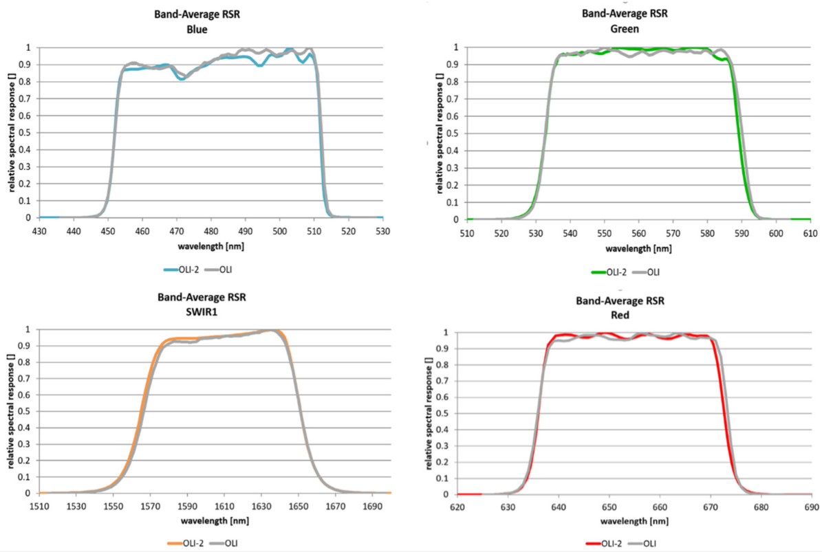
As the spectral filters for OLI and OLI-2 came from the original lot of filters developed for OLI, uncertainty from spectral differences was expected to be quite low. Figure 1 compares the spectral bandpasses, or relative spectral response (RSR) functions, for OLI and OLI-2 for several representative bands. It is clear that differences, though small, do exist.

Figure 1. Representative relative spectral response (RSR) functions for OLI and OLI-2. These are band averages of 14 focal plane modules (FPMs) showing small differences.

To quantify differences that will occur in the sensor outputs due to spectral differences, the well-known spectral band adjustment factor (SBAF) was used. Details on the development and use of SBAF can be found in ^[6]^[7]. Basically, SBAF is the ratio of the reflectance level measured by two sensors that observe the same target simultaneously with the same illumination/viewing geometry, but with differing RSR functions. Any departure from an SBAF value of unity is a direct percentage measurement of the difference in output that would be expected from the sensors.

As SBAF is a function of target type, it was necessary to analyze a large variety of targets to understand the overall impact it would have. Examples of SBAF values for four major representative target types are shown in Figure 2. To obtain spectral information of targets, a variety of spectral databases were utilized: crop information came from the GHISA database ^[8], forest information from the ECOSTRESS library ^[9]^[10], soil information from the ICRAF-ISRIC Library ^[11], and snow information from the National Research Council of Italy Institute of Polar Sciences ^[12]. For all land cover types shown in Figure 2, the SBAF value uncertainties are all less than 1% (deviation from unity < 0.01). For vegetative cases, SBAF values tended to be less than 0.3% for all cases. For the case of soil targets, SBAF can, at worst, be on the order of about 0.7%, but only in the green band. While, for snow, SBAF is much larger than 0.5% in the SWIR. For the case of snow, the driver for the large uncertainty percentages is the low reflectivity of snow in the SWIR ranges. Thus, this can be easily avoided by not using snow-covered targets for cross-calibration of the SWIR bands. The TIRS instrument bands 10 and 11 also have slight differences in the RSRs; however, through multiple simulations with different target types, it was concluded that the SBAF in these bands would be at unity, to within 0.1%. Due to this, spectral uncertainty for TIRS was considered to be negligible for this experiment. In summary, it was felt that, with the judicious use of land cover targets, uncertainty due to spectral differences could be kept well below 0.5%.

Figure 2. SBAFs for all OLI band averages for four common land cover types. (a) is mid-season corn, (b) is White Fir, (c) is Brazilian soil with similar results to that of a desert, and (d) is large rounded grain particles of snow.

2.2. Geometric Uncertainty

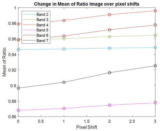
Pointing differences between the two sensors systems were analyzed to determine the degree of uncertainty that would occur for this situation. An analysis was performed using Landsat 7/8 underfly data using pixel shifts between the scene pairs to determine how much any error in pointing would change the cross-calibration ratio. Results from this analysis are shown in Figure 3. In this figure, pixel shift between the images is on the horizontal axis while the resulting ratio of reflectances between the two images is plotted along the vertical axis. As pixel shift increases from zero to three, a small change in the calibration ratio occurs; it is largest in band 7, ranging from approximately 0.895 to 0.925 or a change of about 3.3%. To understand how much shift might occur between Landsat 8 and Landsat 9 images, experts on Landsat geometry were consulted at USGS EROS (Choate, Michael. Interview. Conducted by Dennis Helder, 23 June 2021). Results of that discussion indicated that image-to-image errors would be on the order of 5 m. Since Landsat GSD is 30 m, this represents a pixel shift of 0.16. As can be seen from Figure 3, this leads to a very small change in cross-calibration ratio. Thus, uncertainties due to pointing errors were deemed to be negligible for this application.

Figure 3. Change in cross-calibration ratio as a function of point error. These data were extracted from archived Landsat 7/8 underfly imagery and include the effects of SBAF to minimize spectral error. Thus, changes due to only pointing error will be smaller than values indicated here.

Uncertainty due to differences in viewing/illumination geometry also need to be considered because, during the underfly maneuver, the two sensors have the exact same geometry for only an instant in time. During the course of the maneuver, the sun angle for any given target will be very similar for both sensors, but the viewing angles will change significantly. Worst case, at the beginning and end of the maneuver, when there is minimal image overlap, one sensor will be viewing 7.5° to the west while the other will be viewing 7.5° to the east. Thus, there will be a viewing zenith angle difference (VZAD) of 15°. Since the viewing azimuth angle for the sensors is nominally east/west or, more exactly, nominally 98° and 278° due to the 98° orbital inclination of Landsat, the sensors will be imaging close to the principle plane (that is, the situation where the sensor, target, and sun are contained in a plane) during imaging in the northern hemisphere, and close to the cross-principle plane (orthogonal to the principle plane) in the southern hemisphere, as the sensors complete imaging during the descending portion of the orbit. This geometry occurs because the underfly maneuver occurred on 11–17 November 2021.

2.3. Angular Uncertainty

Even slight differences in viewing and illumination angles when observing a target will result in the sensors capturing slightly different reflectances. Reflectance of surfaces as function of viewing/illumination angle is modeled by target-specific bidirectional reflectance distribution functions (BRDF). Thus, to understand the uncertainty due to viewing angle differences, it was necessary to use a BRDF modeling approach. The Ross–Li BRDF model as used by the MODIS sensors was chosen, since it is broadly accepted by the remote-sensing community and a large amount of data exists ^[13]^[14]^[15]. However, drawbacks of this approach include the fact that the Ross–Li model was developed primarily for vegetation and the spatial resolution of the MODIS sensors is much larger than Landsat’s.

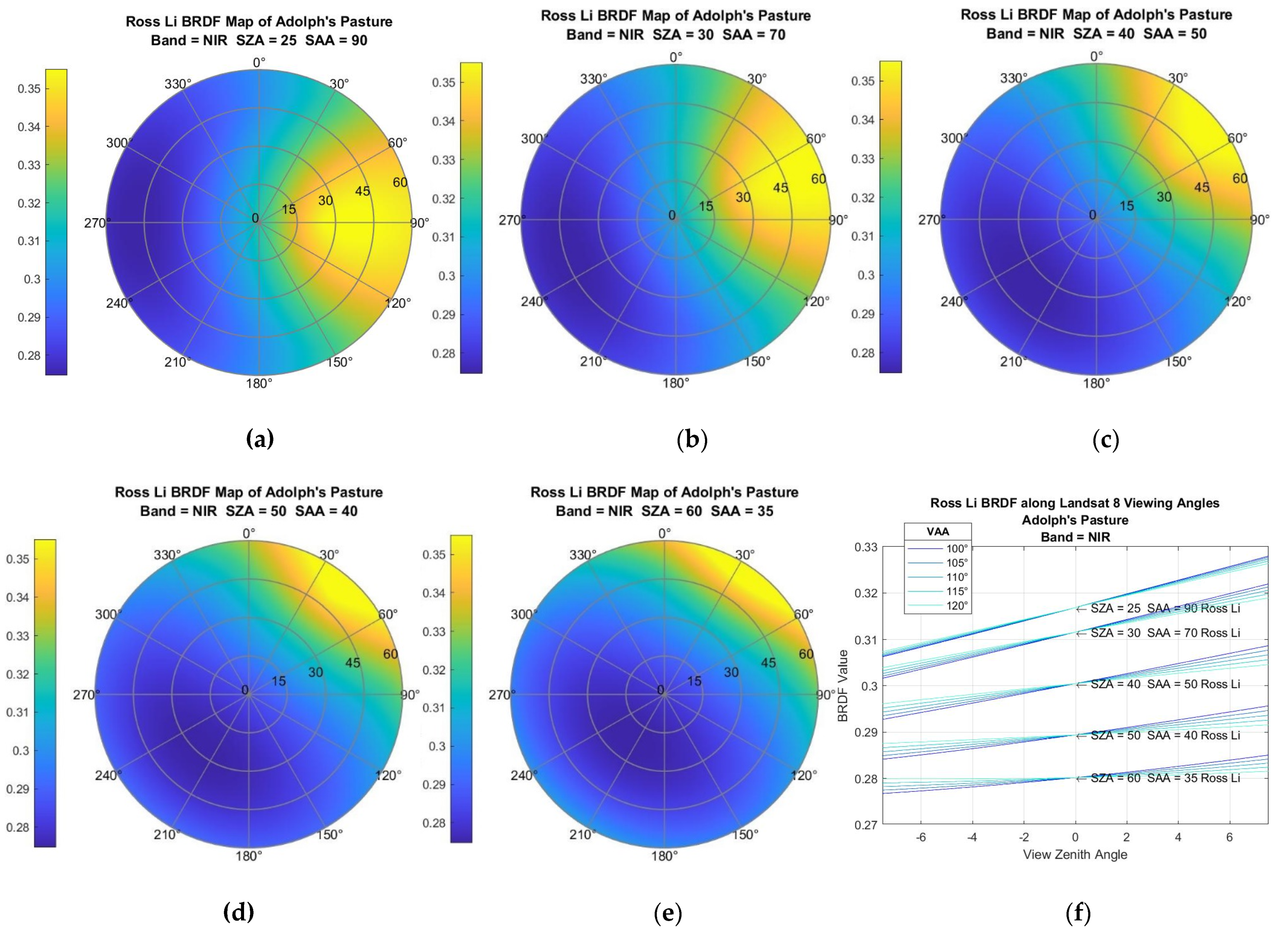
To understand the impact of BRDF on the uncertainty for the underfly maneuver, a simple analysis was performed on two land cover types—a grassy pasture in east central South Dakota (well known to one of the authors) and desert sand (from the well-known Libya 4 calibration site). Examples of the BRDF models obtained from MODIS observations (the MCD43A1 MODIS product) of these locations in summer of 2021 are shown in Figure 4 and Figure 5. From these figures, researchers see that the hot spot (the yellow region indicating higher reflectance) follows the location of the sun azimuthally and moves away from the origin as the SZA increases. Note that Landsat viewing angles are restricted to a region well within the 15° annular ring (±7.5°) and lie along a line roughly from 98° to 278°. If one extracts the data along this line and plots them as a function of VZA, the plot in the lower-right corner of the figure results. The key results to note here are that when VZA is restricted to the narrow range of Landsat angles, the curves are very linear. Secondly, as the VAA moves further from the principal plane, the slope of the lines decreases. Conversely, even for small VZA differences, the change in BRDF becomes large very quickly. Analysis of these VZA differences indicated that when the VZA difference reaches 7°, the change in BRDF value can reach 6% or more depending on SZA and relative azimuth angle. Clearly, BRDF uncertainty is unacceptably large for cross-calibration purposes! Similar results were obtained for the Libya 4 site, which is much more Lambertian in nature than a vegetative site. Figure 5 shows the same type of linear relationship (graph in lower right), and also less sensitivity—in this case, BRDF uncertainty only reached 1.5% at a VZA difference of 7°.

Figure 4. (a–e): BRDF models of grass pasture for different SZA and SAA locations. Note how hot spot follows solar location. (f): Linearity of BRDF versus VZA for entire range of Landsat viewing angles.

Figure 5. (a–e): BRDF models of Libya 4 calibration site for different SZA and SAA locations. Note how hot spot continues to follow solar location, but is more condensed than the previous figure. (f): Linearity of BRDF versus VZA for entire range of Landsat viewing angles. Note these have a smaller slope when compared to the previous figure.

References

Masek, J.G.; Wulder, M.A.; Markham, B.; McCorkel, J.; Crawford, C.J.; Storey, J.; Jenstrom, D.T. Landsat 9: Empowering open science and applications through continuity. Remote Sens. Environ. 2020, 248, 111968.
MarkhamM, B.; McCorkel, J.; Montanaro, M.; Morland, E.; Pearlman, A.; Pedelty, J.; Wenny, B.; Barsi, J.; Donley, E.; Efremova, B.; et al. Landsat 9: Mission Status and Prelaunch Instrument Performance Characterization and Calibration. In Proceedings of the IGARSS 2019—2019 IEEE International Geoscience and Remote Sensing Symposium, Yokohama, Japan, 28 July–2 August 2019; pp. 5788–5791.
Metzler, M.D.; Malila, W.A. Characterization and comparison of Landsat-4 and Landsat-5 Thematic Mapper data. Photogramm. Eng. Remote Sens. 1985, 51, 1315–1330.
Teillet, P.M.; Markham, B.L.; Barker, J.L.; Storey, J.C.; Irish, R.R.; Seiferth, J.C. Landsat sensor cross-calibration using nearly coincidental matching scenes. In Algorithms for Multispectral, Hyperspectral, and Ultraspectral Imagery VI; SPIE: Bellingham, WA, USA, 2000; Volume 4049.
Mishra, N.; Haque, M.O.; Leigh, L.; Aaron, D.; Helder, D.; Markham, B. Radiometric Cross Calibration of Landsat 8 Operational Land Imager (OLI) and Landsat 7 Enhanced Thematic Mapper Plus (ETM+). Remote Sens. 2014, 6, 12619–12638.
Teillet, P.M.; Fedosejevs, G.; Thome, K.J.; Barker, J.L. Impacts of spectral band difference effects on radiometric cross-calibration between satellite sensors in the solar-reflective spectral domain. Remote Sens. Environ. 2007, 110, 393–409.
Chander, G.; Mishra, N.; Helder, D.L.; Aaron, D.; Choi, T.; Angal, A.; Xiong, X. Use of EO-1 Hyperion data to calculate spectral band adjustment factors (SBAF) between the L7 ETM+ and Terra MODIS sensors. In Proceedings of the 2010 IEEE International Geoscience and Remote Sensing Symposium, Honolulu, HI, USA, 25–30 July 2010.
Thenkabail, P.; Aneece, I. Global Hyperspectral Imaging Spectral-Library of Agricultural Crops for Conterminous United States V001 . NASA EOSDIS Land Processes DAAC, 2019. Available online: https://lpdaac.usgs.gov/products/ghisaconusv001 (accessed on 20 March 2021).
Meerdink, S.K.; Hook, S.J.; Roberts, D.A.; Abbott, E.A. The ECOSTRESS spectral library version 1.0. Remote Sens. Environ. 2019, 230, 111196.
Baldridge, A.M.; Hook, S.J.; Grove, C.I.; Rivera, G. The ASTER Spectral Library Version 2.0. Remote Sens. Environ. 2009, 113, 711–715.
World Agroforestry (ICRAF); International Soil Reference and Information Centre (ISRIC). ICRAF-ISRIC Soil VNIR Spectral Library. In World Agroforestry—Research Data Repository, V1; World Agroforestry (ICRAF): Nairobi, Kenya, 2021.
Salvatori, R.; Salzano, R.; Franco, S.D.; Fontinovo, G.; Plini, P. SISpec 2.0 Snow-Ice Spectral Library; National Research Council of Italy, Institute of Polar Sciences: Rome, Italy, 2020.
Wanner, W.; Li, X.; Strahler, A.H. On the derivation of kernels for kernel-driven models of bidirectional reflectance. J. Geophys. Res. Atmos. 1995, 100, 21077–21089.
Wanner, W.; Strahler, A.H.; Hu, B.; Lewis, P.; Muller, J.-P.; Li, X.; Schaaf, C.L.B.; Barnsley, M.J. Global retrieval of bidirectional reflectance and albedo over land from EOS MODIS and MISR data: Theory and algorithm. J. Geophys. Res. Atmos. 1997, 102, 17143–17161.
Lucht, W.; Schaaf, C.B.; Strahler, A.H. An algorithm for the retrieval of albedo from space using semiempirical BRDF models. IEEE Trans. Geosci. Remote Sens. 2000, 38, 977–998.

© Text is available under the terms and conditions of the Creative Commons Attribution (CC BY) license; additional terms may apply. By using this site, you agree to the Terms and Conditions and Privacy Policy.

Upload a video for this entry

Information

Subjects: Remote Sensing

Contributors MDPI registered users' name will be linked to their SciProfiles pages. To register with us, please refer to https://encyclopedia.pub/register :

Garrison Gross

Dennis Helder

Larry Leigh

Morakot Kaewmanee

View Times: 3.1K

Entry Collection: Remote Sensing Data Fusion

Update Date: 01 Jun 2022

Table of Contents

Video Upload Options

Confirm