Atmospheric Turbulence

Version	Summary	Created by	Modification	Content Size	Created at	Operation
1		Albashir Youssef	--	999	2022-04-23 11:54:14	\|
2	format correct	Catherine Yang	-3 word(s)	996	2022-04-24 03:47:13	\|

This entry is adapted from the peer-reviewed paper 10.3390/photonics9040262

The foundation of any smart city requires an innovative and robust communication infrastructure. Many research communities envision free-space optical communication (FSO) as a promising backbone technology for the services and applications provided by such cities. However, the channel through which the FSO signal travels is the atmosphere. Therefore, the FSO performance is limited by the local weather conditions. The variation in meteorological variables leads to variations of the refractive index along the transmission path. These index inhomogeneities (i.e., atmospheric turbulence) can significantly degrade the performance of FSO systems. The effect of atmospheric turbulence on FSO systems is a considerable challenge. Such turbulence can produce beam scintillation, spreading, and wandering, resulting in a significant reduction in BER performance and the inability to use the communication link.

free space optical communication atmospheric turbulence

1. Atmospheric Turbulence

Clear air turbulence can significantly affect the transmitted optical beam. Wind and solar heat can lead to inhomogeneities in the temperature and pressure of air. These variations cause random refractive index fluctuations in the atmosphere, leading to the formation of air cells (eddies) of varying sizes and refractive indexes. Variations in the refractive index and propagation path of the optical beam in air can lead to random fluctuations in both the amplitudes and received signal phase. The block diagram of an FSO communications system is shown in Figure 1. The information signal (analog or digital) is delivered through the atmosphere using an optical transmitter. At the receiver end, the optical beam concentrates towards the photodetector, whose output is electrically processed to receive the information signal. The atmospheric turbulence effect on the optical signal depends on the size of the turbulence cell, which can be defined as follows ^[1]:

/media/item_content/202204/6264a6423adafphotonics-09-00262-g001.png

Figure 1. Comparison of Turbulent Cell Size with (a) Scintillation and (b) Beam Wander.

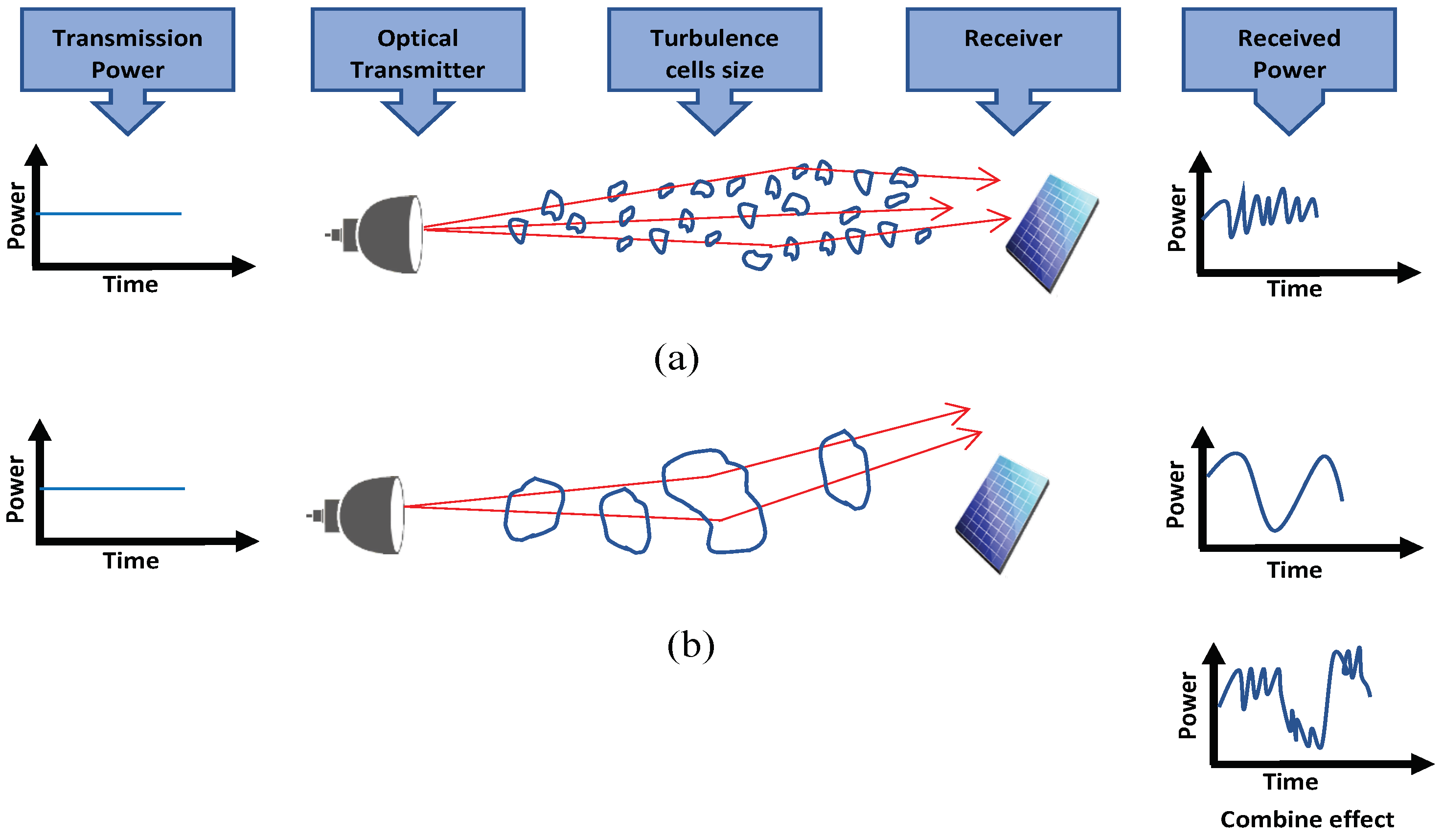
When the turbulence cells’ diameters are smaller than the laser beam diameter, the laser beam bends and becomes distorted. Small differences in the arrival times of various components of the beam wavefront cause constructive and destructive interference, resulting in temporal variations in the laser beam intensity at the receiver. This effect is known as scintillation, Figure 1a.
If the size of the air turbulence cell is larger than the beam diameter, it can bend the optical path. Figure 1b shows how the beams (solid rays) leaving the laser source are deflected as they go through the large air cell, arriving off-axis rather than on-axis as expected in the absence of turbulence.

2. Mathematical Analysis of Atmospheric Turbulence

2.1. Refractive Index Structure Parameter

To determine the strength of atmospheric turbulence, the key aspect is the refractive index of the air,

(C_{n}^{2})

. However, the estimation of

C_{n}^{2}

is an intensive process, owing to the specific hardware and high computation costs involved in this process ^[2]. Several models, such as the Hufnagel‚ Äì-Valley, and Greenwood models are commonly used to predict the refractive index. However, these models are appropriate over a vertical path only ^[2]^[3]. Moreover, the atmospheric turbulence varies with height and local conditions, such as the terrain type, geographical location, and meteorological values ^[4]^[5]. Consequently, it is essential to establish and enhance the

C_{n}^{2}

prediction models using meteorological parameters, such as the temperature, humidity, and wind speed. A macro-meteorological model to estimate

C_{n}^{2}

was adopted.

for the following reasons:

The existing studies demonstrated that the macro-meteorological model can be successfully used to estimate the values of $C_{n}^{2}$ in a coastal area with a high correlation (up to 90%) compared with the measured values ^[5]^[6]^[7]^[8]^[9];

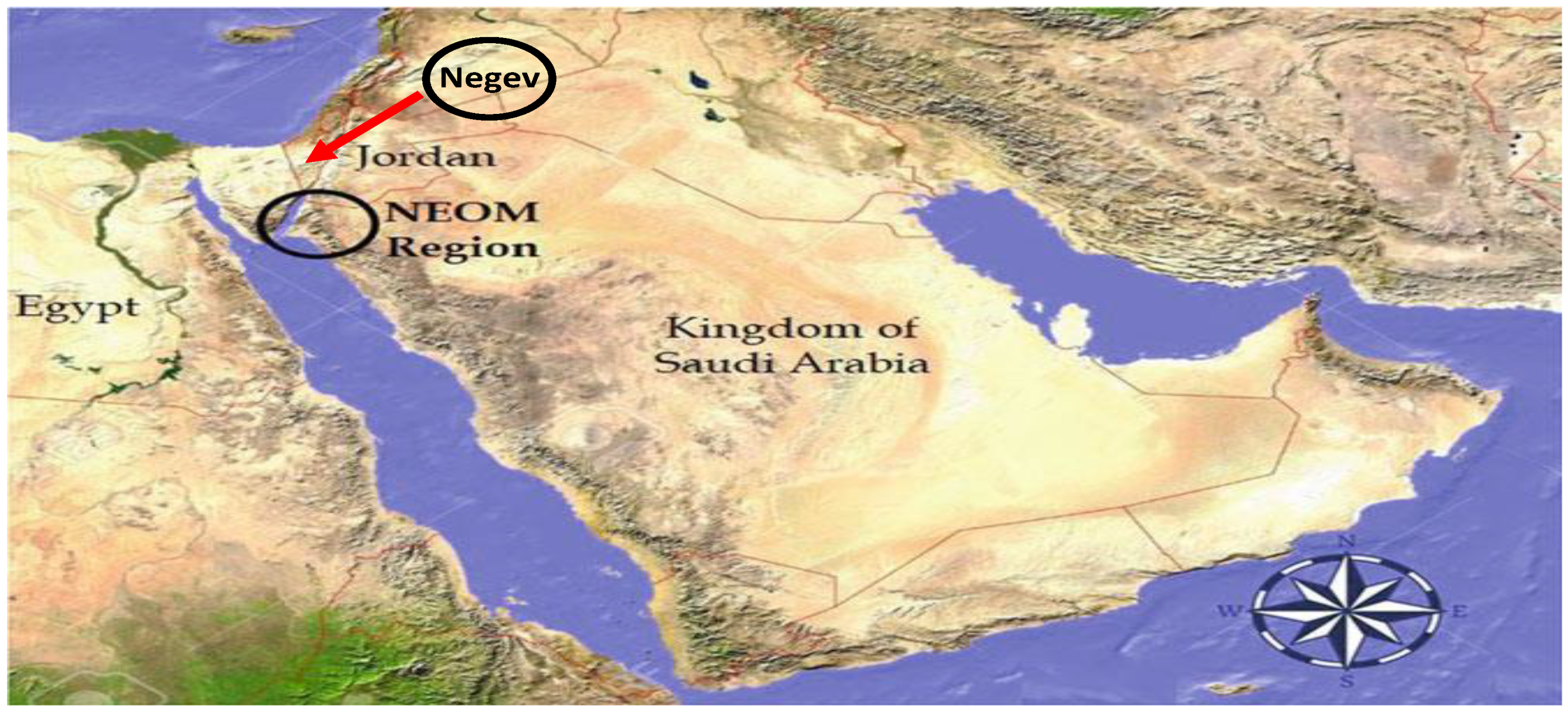
This model has been validated for a similar coastal area called Negev area, as shown in Figure 2. Negev is approximately 400 km from the study area, NEOM, and has a similar landscape;
This model can help correlate the changes in the atmospheric turbulence strength $C_{n}^{2}$ with the meteorological parameters.

/media/item_content/202204/6264a6536e5a9photonics-09-00262-g002.png

Figure 2. Map of Saudi Arabia with the NEOM City Location Marked ^[10].

The macro-meteorological model can be mathematically expressed as ^[11]:

(1)

(2)

(3)

(4)

where W is the weight function, T is the air temperature (° K), H is the relative humidity (%), and v is the wind speed (m/s). This model is valid under specific limits of macroscale parameters, specifically, the temperature (from 9 to 35 °C), relative humidity (from 14% to 92%), and wind speed (from 0 to 10 m/s) ^[11]. The weight function W is calculated based on a temporal hour that relates the actual time to sunrise and sunset, as indicated in Table 1.

(5)

where H_Tis the temporal hour, H_actual is the actual time, H_sunrise is the sunrise time and H_sunset the sunset time. The typical values of $C_{n}^{2}$ are $C_{n}^{2} = 0.5 \times 10^{- 14} m^{- \frac{2}{3}}$ for weak turbulence, $C_{n}^{2} = 2 \times 10^{- 14} m^{- \frac{2}{3}}$ for moderate turbulence, and $C_{n}^{2} = 5 \times 10^{- 14} m^{- \frac{2}{3}}$ for strong turbulence ^[12]^[13].

Table 1. Weight Function ^[11].

Temporal Hour Interval	W	Temporal Hour Interval	W
Until −4	0.11	5 to 6	1.00
−4 to −3	0.11	6 to 7	0.90
−3 to −2	0.07	7 to 8	0.80
−2 to −1	0.08	8 to 9	0.59
−1 to 0	0.06	9 to 10	0.32
Sunrise 0 to 1	0.05	10 to 11	0.22
1 to 2	0.10	11 to 12	0.10
2 to 3	0.51	12 to 13	0.08
3 to 4	0.75	Over 13	0.13
4 to 5	0.95

2.2. Scintillation

Scintillation is described as the temporal and spatial fluctuation of the light intensity caused by atmospheric turbulence. The scintillation index,

σ_{I}^{2}

, is defined as the normalized variance of the light wave intensity:

(6)

where I is a time series of intensity measurements, and the angle brackets denote a time average. The relation between the refractive index structure parameter and $σ_{I}^{2}$ is ^[14]

(7)

where $k = 2 π / λ$ represents the wave number, λ is the wavelength, and L is the transmission distance. The scintillation index is commonly used to classify intensity fluctuation, and its values for weak, moderate, and strong fluctuations are $σ_{I} < 1$ , $σ_{I} \sim 1$ , and $σ_{I} > 1$ , respectively ^[14]. Generally, scintillation can result in a high BER.

2.3. Beam Spreading

When a beam propagates through the turbulent atmosphere, beam spreading which is defined as the broadening of the beam at the receiver surface beyond vacuum diffraction, occurs. The researchers describe the Gaussian beam spreading of a beam propagating through turbulence at a distance L from the source. To estimate the amount of beam spreading, the effective average beam waist,

w_{e f f} (L)

, is defined as follows ^[1]:

(8)

where $w (L)$ is the beam waist at a propagation distance L.

(9)

where $w_{0}$ is the initial beam waist at $L = 0$ .

References

Alkholidi, A.; Altowij, K. Effect of Clear Atmospheric Turbulence on Quality of Free space Optical Communications in Western Asia. Opt. Commun. Syst. 2012, 1, 41–72.
Raj, A.A.B.; Selvi, J.A.V.; Durairaj, S. Comparison of Different Models for Ground-Level Atmospheric Turbulence Strength ( C n 2 ) Prediction with A New Model According to Local Weather Data for FSO Applications. Appl. Opt. 2015, 54, 802–815.
Wilcox, C.C.; Restaino, S.R. A New Method of Generating Atmospheric Turbulence with A Liquid Crystal Sspatial Light Modulator; THI Sone Is: A Chapter in New Development in Liquid Crystals; InTech: Toyama, Toyama, 2009; ISBN 978-953-307-015-5.
Sadot, D.; Kopeika, N.S. Forecasting Optical Turbulence Strength on the Basis of Macroscale Meteorology and Aerosols: Models and Validation. Opt. Eng. 1992, 31, 200–212.
Bendersky, S.; Kopeika, N.S.; Blaunstein, N. Atmospheric Optical Turbulence over Land in Middle East Coastal Environments: Prediction Modeling and Measurements. Appl. Opt. 2004, 43, 4070–4079.
Lionis, A.; Peppas, K.; Nistazakis, H.E.; Tsigopoulos, A.; Cohn, K. Statistical Modeling of Received Signal Strength for An FSO Link over Maritime Environment. Opt. Commun. 2021, 489, 126858.
Wang, H.; Li, B.; Wu, X.; Liu, C.; Hu, Z.; Xu, P. Prediction Model of Atmospheric Refractive Index Structure Parameter in Coastal Area. J. Mod. Opt. 2015, 62, 1336–1346.
Bendersky, S.; Lilos, E.; Kopeika, N.S.; Blaunstein, N. Modeling and Measurements of Near-Gground Atmospheric Optical Turbulence According to Weather for Middle East Environments. In Proceedings of the SPIE 5612, Electro-Optical and Infrared Systems: Technology and Applications, London, UK, 6 December 2004.
Jellen, C.; Nelson, C.; Brownell, C.; Burkhardt, J.; Oakley, M. Measurement and Analysis of Atmospheric Optical Turbulence in A Near-Maritime Environment. IOP SciNotes 2020, 1, 024006.
Saud, M.M.A. Sustainable Land Management for NEOM Region; Springer: Berlin/Heidelberg, Germany, 2020.
Porras, R.B. Exponentiated Weibull Fading Channel Model in Free-Space Optical Communications Under Atmospheric Turbulence. Ph.D. Dissertation, Universitat Politecnica de Catalunya, Barcelona, Spain, 2013.
Farid, A.A.; Hranilovic, S. Outage Capacity Optimization for Free-Space Optical Links with Pointing Errors. J. Light. Technol. 2007, 25, 1702–1710.
Abaza, M.; Mesleh, R.; Mansour, A.; Aggoune, E.-H.M. Relay Selection for Full-Duplex FSO Relays over Turbulent Channels. In Proceedings of the the 16TH IEEE International Symposium on Signal Processing and Information Technology (ISSP 2016), Limassol, Cyprus, 12–14 December 2016.
Zhangy, M.; Tang, X.; Lin, B.; Ghassemlooy, Z.; Wei, Y. Analysis of Rytov Variance in Free Space Optical Communication under the Weak Turbulence. In Proceedings of the 16th International Conference on Optical Communications and Networks (ICOCN), Wuzhen, China, 7–10 August 2017.

© Text is available under the terms and conditions of the Creative Commons Attribution (CC BY) license; additional terms may apply. By using this site, you agree to the Terms and Conditions and Privacy Policy.

Upload a video for this entry

Information

Subjects: Engineering, Electrical & Electronic

Contributors MDPI registered users' name will be linked to their SciProfiles pages. To register with us, please refer to https://encyclopedia.pub/register :

Albashir Youssef

Ayshah Alatawi

Mohamed Abaza

Mohammad Ashfaq

Ali MANSOUR

View Times: 1.4K

Entry Collection: Environmental Sciences

Update Date: 24 Apr 2022

Table of Contents

Video Upload Options

Confirm