Atmospheric Turbulence | Encyclopedia MDPI

Atmospheric Turbulence: History

View Latest Version

Please note this is an old version of this entry, which may differ significantly from the current revision.

Subjects: Engineering, Electrical & Electronic

Contributor:

The foundation of any smart city requires an innovative and robust communication infrastructure. Many research communities envision free-space optical communication (FSO) as a promising backbone technology for the services and applications provided by such cities. However, the channel through which the FSO signal travels is the atmosphere. Therefore, the FSO performance is limited by the local weather conditions. The variation in meteorological variables leads to variations of the refractive index along the transmission path. These index inhomogeneities (i.e., atmospheric turbulence) can significantly degrade the performance of FSO systems. The effect of atmospheric turbulence on FSO systems is a considerable challenge. Such turbulence can produce beam scintillation, spreading, and wandering, resulting in a significant reduction in BER performance and the inability to use the communication link.

free space optical communication
atmospheric turbulence

1. Atmospheric Turbulence

Clear air turbulence can significantly affect the transmitted optical beam. Wind and solar heat can lead to inhomogeneities in the temperature and pressure of air. These variations cause random refractive index fluctuations in the atmosphere, leading to the formation of air cells (eddies) of varying sizes and refractive indexes. Variations in the refractive index and propagation path of the optical beam in air can lead to random fluctuations in both the amplitudes and received signal phase. The block diagram of an FSO communications system is shown in Figure 1. The information signal (analog or digital) is delivered through the atmosphere using an optical transmitter. At the receiver end, the optical beam concentrates towards the photodetector, whose output is electrically processed to receive the information signal. The atmospheric turbulence effect on the optical signal depends on the size of the turbulence cell, which can be defined as follows [39]:

Figure 1. Comparison of Turbulent Cell Size with (a) Scintillation and (b) Beam Wander.

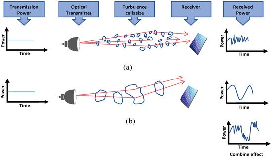
When the turbulence cells’ diameters are smaller than the laser beam diameter, the laser beam bends and becomes distorted. Small differences in the arrival times of various components of the beam wavefront cause constructive and destructive interference, resulting in temporal variations in the laser beam intensity at the receiver. This effect is known as scintillation, Figure 1a.
If the size of the air turbulence cell is larger than the beam diameter, it can bend the optical path. Figure 1b shows how the beams (solid rays) leaving the laser source are deflected as they go through the large air cell, arriving off-axis rather than on-axis as expected in the absence of turbulence.

2. Mathematical Analysis of Atmospheric Turbulence

2.1. Refractive Index Structure Parameter

To determine the strength of atmospheric turbulence, the key aspect is the refractive index of the air,(C2n) However, the estimation of C2n is an intensive process, owing to the specific hardware and high computation costs involved in this process [40]. Several models, such as the Hufnagel‚ Äì-Valley, and Greenwood models are commonly used to predict the refractive index. However, these models are appropriate over a vertical path only [40,41]. Moreover, the atmospheric turbulence varies with height and local conditions, such as the terrain type, geographical location, and meteorological values [42,43]. Consequently, it is essential to establish and enhance the C2n prediction models using meteorological parameters, such as the temperature, humidity, and wind speed. In this study, we adopt a macro-meteorological model to estimate C2n

for the following reasons:

The existing studies demonstrated that the macro-meteorological model can be successfully used to estimate the values of $C_{n}^{2}$

in a coastal area with a high correlation (up to 90%) compared with the measured values [43,44,45,46,47];
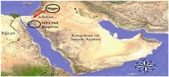
This model has been validated for a similar coastal area called Negev area, as shown in Figure 2. Negev is approximately 400 km from the study area, NEOM, and has a similar landscape;
This model can help correlate the changes in the atmospheric turbulence strength $C_{n}^{2}$

with the meteorological parameters.

Figure 2. Map of Saudi Arabia with the NEOM City Location Marked [51].

The macro-meteorological model can be mathematically expressed as [48]:

(1)

(2)

(3)

(4)

where W is the weight function, T is the air temperature (° K), H is the relative humidity (%), and v is the wind speed (m/s). This model is valid under specific limits of macroscale parameters, specifically, the temperature (from 9 to 35 °C), relative humidity (from 14% to 92%), and wind speed (from 0 to 10 m/s) [48]. The weight function W is calculated based on a temporal hour that relates the actual time to sunrise and sunset, as indicated in Table 1.

(5)

where HT is the temporal hour, Hactual is the actual time, Hsunrise is the sunrise time and Hsunset the sunset time. The typical values of C2n are C2n=0.5×10−14m−23 for weak turbulence, C2n=2×10−14m−23 for moderate turbulence, and C2n=5×10−14m−23

for strong turbulence [49,50].

Table 1. Weight Function [48].

Temporal Hour Interval	W	Temporal Hour Interval	W
Until −4	0.11	5 to 6	1.00
−4 to −3	0.11	6 to 7	0.90
−3 to −2	0.07	7 to 8	0.80
−2 to −1	0.08	8 to 9	0.59
−1 to 0	0.06	9 to 10	0.32
Sunrise 0 to 1	0.05	10 to 11	0.22
1 to 2	0.10	11 to 12	0.10
2 to 3	0.51	12 to 13	0.08
3 to 4	0.75	Over 13	0.13
4 to 5	0.95

4.2. Scintillation

Scintillation is described as the temporal and spatial fluctuation of the light intensity caused by atmospheric turbulence. The scintillation index,

σ_{I}^{2}

, is defined as the normalized variance of the light wave intensity:

(6)

where I is a time series of intensity measurements, and the angle brackets denote a time average. The relation between the refractive index structure parameter and σ2I is [52]

(7)

where k=2π/λ represents the wave number, λ is the wavelength, and L is the transmission distance. The scintillation index is commonly used to classify intensity fluctuation, and its values for weak, moderate, and strong fluctuations are σI<1, σI∼1, and σI>1

, respectively [52]. Generally, scintillation can result in a high BER.

4.3. Beam Spreading

When a beam propagates through the turbulent atmosphere, beam spreading which is defined as the broadening of the beam at the receiver surface beyond vacuum diffraction, occurs. In this section, we describe the Gaussian beam spreading of a beam propagating through turbulence at a distance L from the source. To estimate the amount of beam spreading, the effective average beam waist,

w_{e f f} (L)

, is defined as follows [39]:

(8)

where w(L) is the beam waist at a propagation distance L.

(9)

where w0 is the initial beam waist at L=0 m.

This entry is adapted from the peer-reviewed paper 10.3390/photonics9040262

© Text is available under the terms and conditions of the Creative Commons Attribution (CC BY) license; additional terms may apply. By using this site, you agree to the Terms and Conditions and Privacy Policy.