Hyperspectral Remote Sensing

Version	Summary	Created by	Modification	Content Size	Created at	Operation
1		NURSYAZYLA SULAIMAN	+ 2237 word(s)	2237	2022-03-08 09:54:09	\|
2	format correction	Peter Tang	Meta information modification	2237	2022-03-18 03:31:47	\|

This entry is adapted from the peer-reviewed paper 10.3390/app12052570

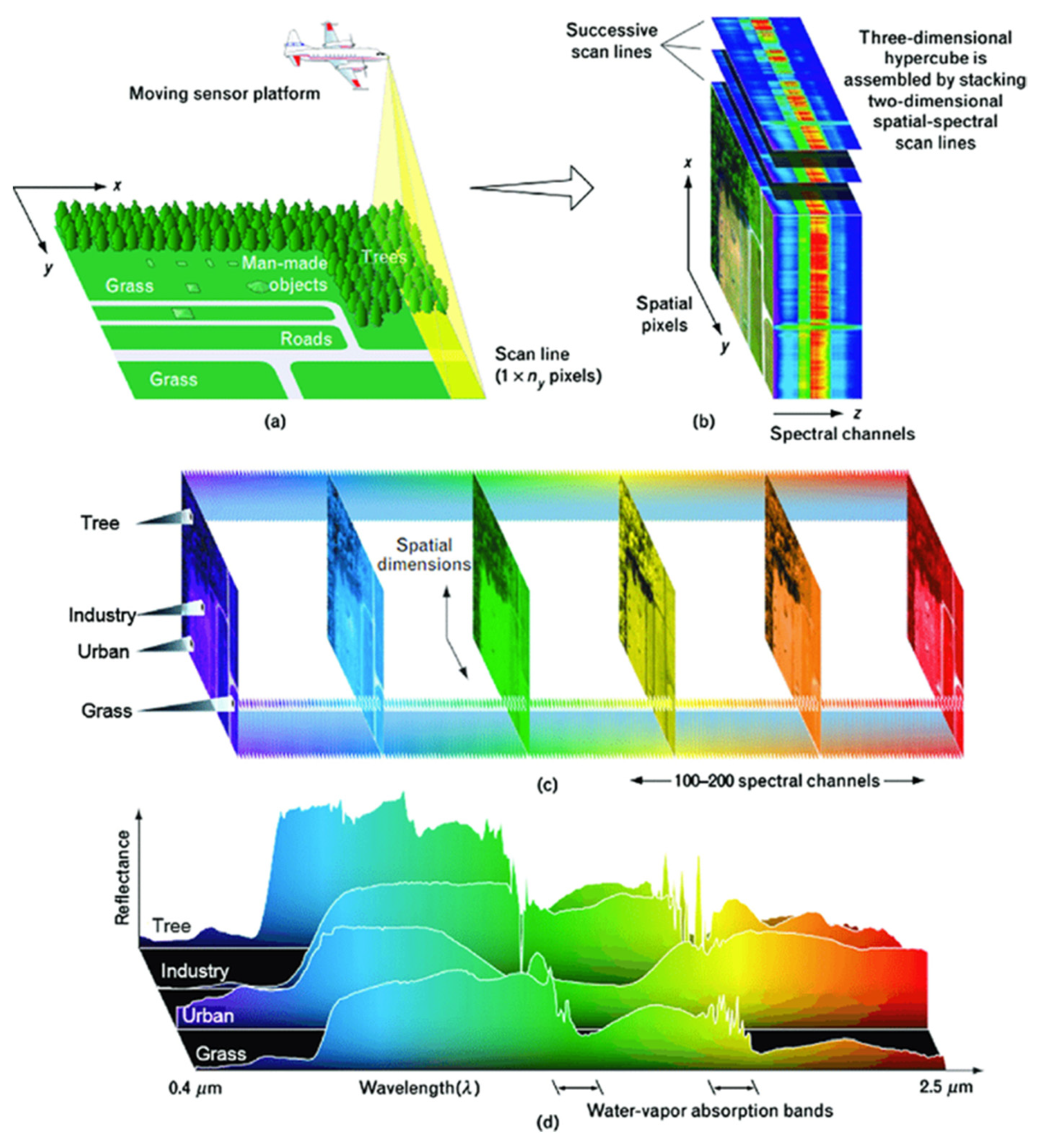
Hyperspectral imaging is an incorporation of the modern imaging system and traditional spectroscopy technology. Unmanned aerial vehicle (UAV) hyperspectral imaging techniques have recently emerged as a valuable tool in agricultural remote sensing, with tremendous promise for many application such as weed detection and species separation

hyperspectral imagery remote sensing

1. Hyperspectral Remote Sensing: A Brief Overview

According to Weiss et al. ^[1], agriculture monitoring from remote sensing is a vast subject that has been widely addressed from multiple perspectives, sometimes based on specific applications (e.g., precision farming, yield prediction, irrigation, weed detection), remote sensing platforms (e.g., satellites, unmanned aerial vehicles—UAVs, unmanned ground vehicles—UGVs), or sensors (e.g., active or passive sensing, wavelength domain) or specific locations and climatic contexts (e.g., country or continent, wetlands or drylands). Campbell and Wynne ^[2] defined remote sensing as the application of acquiring information regarding the Earth’s land and water surface by utilising images obtained from an overhead perspective, implementing electromagnetic radiation in one or more regions of the electromagnetic spectrum, reflected or emitted from the Earth’s surface. Hyperspectral remote sensing involves extracting information from the objects or scenes that lie on the Earth’s surface due to radiance obtained by airborne or spaceborne sensors ^[3]^[4].

Generally, hyperspectral imaging is an incorporation of the modern imaging system and traditional spectroscopy technology ^[5]^[6]. According to Govender et al. ^[7], the evolution of airborne and satellite hyperspectral sensor technologies has overcome the restraint of multispectral sensors since hyperspectral sensors assemble several narrow spectral bands from the visible, near-infrared (NIR), mid-infrared, and short-wave infrared portions of the electromagnetic spectrum. The hyperspectral sensor collects about 200 or more spectral bands, each only 10 nm wide ^[2] which allows the construction of continuous spectral reflectance signatures while the narrow bandwidths element of hyperspectral data enable in-depth examination of Earth surface characteristics which would disappear within the relatively coarse bandwidths acquired with multispectral data. Hyperspectral data are usually assigned as hypercubes (see Figure 1) that contain two spatial dimensions and one spectral dimension, regarding the characteristics of each hyperspectral image, comprising many channels since there were bands—in contrast to grayscale or RGB images—that included only one or three channels, respectively ^[8].

/media/item_content/202203/6233eedcdb16dapplsci-12-02570-g001.png

Figure 1. Hyperspectral data cube structure ^[9]^[10].

The hyperspectral data cube in Figure 1 explained that Figure 1a A push-broom sensor on an airborne or spaceborne platform acquire spectral data for a one-dimensional row of cross-track pixels named as scanline; Figure 1b Sequential scan lines including spectra for each row of cross-track pixels are pilled to obtain a three-dimensional hyperspectral data cube which in this illustration the spatial details of a scene are constituted by the x and y dimensions of the cube, while the amplitude spectra of the pixels are projected to the z dimension; Figure 1c the three-dimensional hyperspectral data cube can be analysed as a stack of two-dimensional spatial images whereas each is equivalent to a particular narrow waveband. Usually, hyperspectral data cubes contain hundreds of stacked images; Figure 1d the spectral samples can be marked for each pixel and discrimination of the features in the spectra deliver the primary mechanism for detection and classification in a scene ^[9]^[10]. Qian ^[6] stated that there were about three different methods in obtaining the hyperspectral data regarding the type of imaging spectrometers such as dispersive elements-based approach, spectral filters-based approach and snapshot hyperspectral imaging. In order to collect the hyperspectral images with different spatial and temporal resolutions, the sensors used can, for example, be mounted on different platforms. Unmanned-aerial vehicles (UAVs), airplanes, and close-range platforms ^[11]. Table 1 shows the comparison of different types of hyperspectral imaging platforms. Kate et al. ^[12] mentioned that hyperspectral sensors were utilised for providing information such as airborne visible/infrared imaging spectrometer (AVIRIS), Hyperion, Hymap (from HyVista Castle Hill, Australia), and airborne imaging spectroradiometer for applications (AISA). Table 2 below shows different types of hyperspectral sensors used which are usually mounted on the aircraft and satellite ^[13].

Table 1. Comparison of hyperspectral imaging platforms ^[11].

Parameters	Satellites	Airplanes	Helicopters	Fixed-Wing UAVs	Multi-Rotor UAVs	Close-Range Platforms
Operational Altitudes	400–700 km	1–20 km	100 m–2 km	<150 m	<150 m	<10 m
Spatial coverage	42 km × 7.7 km	~100 km²	~10 km²	~5 km²	~0.5 km²	~0.005 km²
Spatial resolution	20–60 m	1–20 m	0.1–1 m	0.01–0.5 m	0.01–0.5 m	0.0001–0.01 m
Temporal resolution	Days to weeks	Depends on flight operations (hours to days)
Flexibility	Low (fixed by repeating cycles)	Medium (depend on availability of aviation company)		High
Operational complexity	Low (provide final data to users)	Medium (depend on users or vendors)		High (operate by users with setting up the hardware and software)
Applicable scales	Regional–global	Landscape-regional		Canopy–landscape		Leaf–canopy
Major limiting factors	Weathers	Unfavourable flight height/speed, unstable illumination conditions		Short battery endurance, flight regulations		Platform design and operation
Image acquisition cost	Low to medium	High (typically need to hire an aviation company to fly)		Large (due to area coverage)

Table 2. Type of hyperspectral sensors on aircraft and satellites ^[13].

Types of Sensors	Producer	Number of Bands	Spectral Image (μm)
Satellite mounted hyperspectral sensors
FTHSI on MightySat II	Air Force Research (OH, USA)	256	0.35–1.05
Hyperion on EO-	NASA Guddard Space Flight Center (Greenbelt, MA, USA)	242	0.40–250
Aircraft-mounted hyperspectral sensors
AVIRIS (airborne visible infrared imaging spectrometer)	NASA Jet Propulsion Lab. (Pasadena, CA, USA)	224	0.40–2.50
HYDICE (hyperspectral digital imagery collection experiment)	Naval Research Lab (Washington, DC, USA)	210	0.40–2.50
PROBE-1	Earth Search Sciences Inc. (Kalispell, MT, USA)	128	0.40–2.50
CASI (compact airborne spectrographic imager)	ITRES Research Limited (Calgary, AB, Canada)	Over 22	0.40–1.00
HyMap	Integrated Spectronics	100 la 200	Visible to thermal Infrared
EPS-H (environmental protection system)	GER Corporation	VIS/NIR (76), SWIR1 (32), SWIR2 (32), TIR (12)	VIS/NIR (0.43–1.05) SWIR1 (1.50–1.80) SWIR2 (2.00–2.50) TIR (8–12.50)
DAIS 7915 (digital airborne imaging spectrometer)	GER Corporation (geophysical and environmental research imaging spectrometer)	VIS/NIR (32), SWIR1 (8), SWIR2 (32), MIR (1), TIR (12)	VIS/NIR (0.43–1.05) SWIR1 (1.50–1.80) SWIR2 (2.00–2.50) MIR (3.00–5.00) TIR (8.70–12.30)
DAIS 21115 (digital airborne imaging spectrometer)	GER Corporation	VIS/NIR (76), SWIR1 (64), SWIR2 (64), MIR (1), TIR (6)	VIS/NIR (0.40–1.00) SWIR1 (1.00–1.80) SWIR2 (2.00–2.50) MIR (3.00–5.00) TIR (8.00–12.00)
AISA (airborne imaging spectrometer)	Spectral Imaging	Over 288	0.43–1.00

2. Hyperspectral Remote Sensing Imagery (HRSI) Data Processing and Analysing

2.1. Data Preprocessing

According to Weng and Xiaofei ^[14], due to the high-dimensional nature of hyperspectral data, as well as the resemblance between the spectra and mixed pixels, hyperspectral image technology still confronts a number of issues, the most pressing of which are the following: (1) Hyperspectral image data have high dimensionality. Because hyperspectral images are created by combining hundreds of bands of spectral reflectance data gathered by airborne or space-borne imaging spectrometers, the spectrum information dimension of hyperspectral images can also be hundreds of dimensions; (2) missing labelled samples. In practical applications, collecting hyperspectral image data is rather simple, but obtaining image-like label information is quite challenging. As a result, the categorization of hyperspectral pictures is sometimes hampered by a shortage of labelled samples; (3) variability in spectral information across space. The spectral information of hyperspectral images changes in the spatial dimension as a result of factors such as atmospheric conditions, sensors, the composition and distribution of ground features, and the surrounding environment, resulting in the ground feature corresponding to each pixel not being single; and lastly (4) image quality which is the interference of noise and background elements during the acquisition of hyperspectral pictures which has a significant impact on the quality of the data collected. The categorization accuracy of hyperspectral images is directly influenced by the image quality.

Hyperspectral images obtained by various platforms and sensors are usually presented in raw format which requires them to be pre-processed (for example, atmospheric, radiometric, and spectral corrections) to rectify detailed information ^[11]. Assembling hyperspectral data is more intricate than multispectral and RGB sensors because its radiometric and atmospheric calibration workflows are more involuted ^[15]. Therefore, several steps were required for the hyperspectral imaging processing procedure in order to obtain precise output ^[8]. The processing of hyperspectral imaging signifies the utilisation of computer algorithms. It includes tasks such as extracting, storing and falsifying information from visible near-infrared (VNIR) or near-infrared (NIR) hyperspectral images. It also provides different information on processing and data mining assignments (for example, analyse, classify, target detection, regression, and pattern identification) ^[16]^[17]. Hyperspectral imaging includes extensive data collection stored in pixels while each data particularly correlates to their neighbours ^[18]. Hyperspectral imaging also comprises the spectral-domain signal as each of the image pixels contains the spectral information; thus, specific tools and approaches have been amplified for processing both spatial and spectral information ^[17]. This magnitude of data has led to the integration of chemometric and visualisation equipment to competently mine for significant and detailed information ^[19]. The ordinary hyperspectral image preprocessing procedure is delineated in Figure 2 below ^[17].

Figure 2. Hyperspectral image preprocessing workflow ^[17].

According to Burger and Geladi ^[20], numerous amounts of raw data produced from hyperspectral imaging devices contain lots of errors that can be rectified by calibration. Spatial calibration is one of the steps that correlates each image pixel to known units or features, bestowing information about the spatial dimensions and also rectifying the optical aberrations (smile and keystone effects) ^[17]. However, three conditions could prevail which invalidate calibration models which are: (1) chemical or physical substitution in samples, (2) change of equipment due to inherent uncertainty or ageing parts and, (3) environment/weather condition, for example, temperature or humidity ^[21]. Lu et al. ^[11] mentioned that hundreds of bands are common in hyperspectral photographs, and many of them are highly connected. As a result, dimension reduction is an important step to consider while pre-processing hyperspectral images. Dimensionality reduction is a crucial pre-processing step in hyperspectral image classification that reduces HSI’s spectral redundancy, resulting in faster processing and higher classification accuracy. Methods for reducing dimensionality convert high-dimensional data into a low-dimensional space while keeping spectral information ^[22]. Hence, pre-processing is an important step in increasing the quality of hyperspectral images and preparing them for subsequent analysis.

Basantia et al. ^[23] stated that hyperspectral imaging generates extensive data collection from a single sample and with thousands of samples that require daily analysis. According to Tamilarasi and Prabu ^[24], in contrast to other statistical techniques, hyperspectral image analysis uses physical and biological models to absorb light at certain wavelengths. For example, air gases and aerosols could absorb light at specific wavelengths. Dispersion (adding an outside light source to the sensor region of perspective) and absorption are examples of atmospheric diminution (radiance denial). As the outcome, a hyperspectral sensor could not differentiate the radiance recorded with the imaging generated at other times or locations. Hyperspectral image analysis techniques are derived from spectroscopy, which relates to the distinct absorption or patterns of reflection of the context at different wavelengths of a certain material’s molecular composition. This image must be subjected to appropriate atmospheric correction techniques in order to compare each pixel’s reflection signature to the spectrum of known material; in laboratories and in “library” storage areas, known spectral information of materials include soils, minerals and vegetation types.

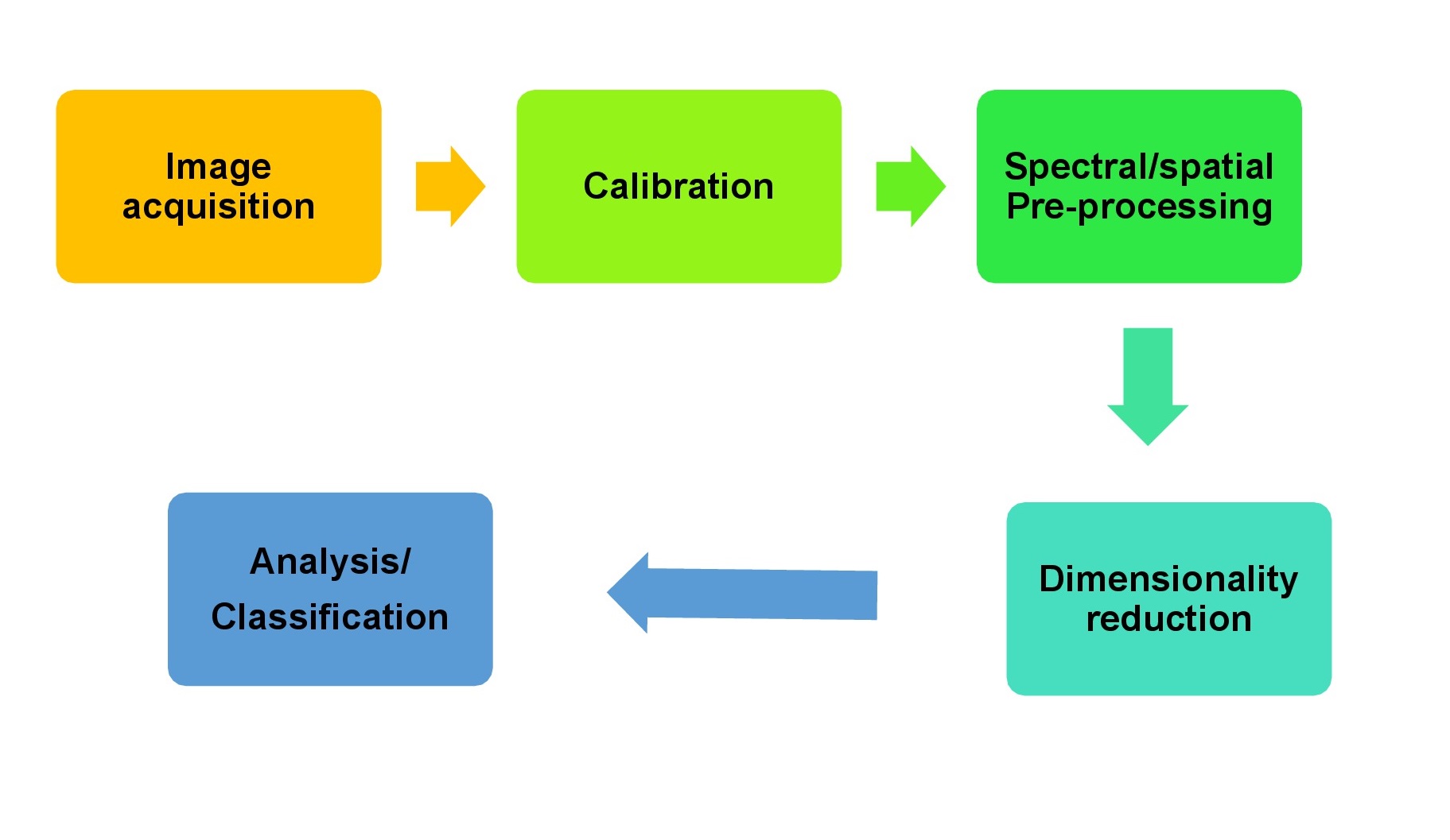
2.2. Hyperspectral Image Classification

Hyperspectral imaging (HSI) is classified as supervised, unsupervised, and semi-supervised based on the nature of available training samples. The supervised technique uses ground truth information (labelled data) for classification whereas the unsupervised technique does not require any prior information ^[25]. According to Wenjing and Xiaofei ^[14], support vector machines, artificial neural networks, decision trees and maximum likelihood classification methods are examples of commonly used supervised classification methods. The basic process is to first determine the discriminant criteria based on the known sample category and prior knowledge and then calculate the discriminant function. Therefore, in supervised classification, Freitas et al. ^[26] stated that support vector machines can produce results that are similar to neural networks but at a lower computing cost and faster rate, making them ideal for hyperspectral data analysis.

Unsupervised classification refers to categorization based on hyperspectral data spectral similarity, for example, clustering without prior knowledge. As stated by Wenjing and Xiaofei ^[14], unsupervised classification can only assume beginning parameters, build clusters through pre-classification processing, and then iterate until the relevant parameters reach the permitted range since no prior knowledge is employed. Examples of unsupervised classification are K-means classification and the iterative self-organizing method (ISODATA). Lastly, is the semi-supervised classification which trains the classifier using both labelled and unlabelled data. The semi-supervised learning paradigm has been successfully utilized beyond hyperspectral imaging ^[27]. It compensates for the lack of both unsupervised and supervised learning opportunities. On the feature space, this classification approach uses the same type of labelled and unlabelled data. Because a large number of unlabelled examples may better explain the overall properties of the data, the classifier trained using these two samples has superior generalisation. Examples of semi-supervised classification are Laplacian support vector machine (LapSVM) and self-training ^[14].

Therefore, hyperspectral imaging can be one of the potential techniques for automatic discriminations between crops and weeds. These sensing technologies have been utilized in smart agriculture and made substantial progress by generating large amounts of data from the fields. Machine learning modelling integrating features has also accomplished reasonable accuracy in order to identify whether a plant is a weed or a crop. Table 3 shows the application of hyperspectral imaging for the discrimination of crops from weeds by using machine learning.

Table 3. Hyperspectral imaging for discrimination of crops from weeds using machine learning ^[28].

No.	Crop	Weed	Model	Optimal Accuracy	Reference
1.	Rice	Barnyard grass, weedy rice	RF, SVM	100%	Zhang et al. (2019)
2.	Maize	Caltrop, curly dock, barnyard grass, ipomoea spp., polymeria spp.	SVM, LDA	>98.35%	Wendel et al. (2016)
3.	Soybean, cotton	Ryegrass	LDA	>90%	Huang et al. (2016)
4.	Wheat	Broadleaf weeds, grass weeds	PLSDA	85%	Hermann et al. (2013)
5.	Broadbean, wheat	Cruciferous weeds	ANN	100%	De Castro et al. (2012)
6.	Sugar beet	Wild buckwheat, Field Horsetail, Green foxtail, Chickweed	LDA	97.3%	Okamoto et al. (2007)
7.	Wheat	Musk thistle	SVM	91%	Mirik et al. (2013)
8.	Maize	C. arvenis	RF	>90%	Gao et al. (2018)

RF—random forest; SVM—support vector machines; LDA—linear discriminant analysis; ANN—artificial neural network; PLSDA—partial least square discriminant analysis.

References

Weiss, M.; Jacob, F.; Duveiller, G. Remote sensing for agricultural applications: A meta-review. Remote Sens. Environ. 2020, 236, 111402.
Campbell, J.B.; Wynne, R.H. Introduction to Remote Sensing; Guilford Press: New York, NY, USA, 2011.
Bioucas-Dias, J.M.; Plaza, A.; Camps-Valls, G.; Scheunders, P.; Nasrabadi, N.M.; Chanussot, J. Hyperspectral remote sensing data analysis and future challenges. IEEE Geosci. Remote Sens. Mag. 2013, 1, 6–36.
Camps-Valls, G.; Tuia, D.; Gómez-Chova, L.; Jiménez, S.; Malo, J. Remote sensing image processing. Synth. Lect. Image Video Multimed. Process. 2011, 5, 1–192.
Qian, S.-E. Optical Satellite Signal Processing and Enhancement; SPIE Press: Bellingham, DC, USA; Cardiff, Wales, 2013.
Qian, S.E. Hyperspectral Satellites and System Design; CRC Press: Boca Raton, FL, USA, 2020.
Govender, M.; Chetty, K.; Naiken, V.; Bulcock, H. A comparison of satellite hyperspectral and multispectral remote sensing imagery for improved classification and mapping of vegetation. Water SA 2019, 34, 147.
Wendel, A. Hyperspectral Imaging from Ground Based Mobile Platforms and Applications in Precision Agriculture; School of Aerospace, Mechanical and Mechatronic Engineering, The University of Sydney: Sydney, Australia, 2018.
Chen, Y.; Guerschman, J.; Cheng, Z.; Guo, L. Remote sensing for vegetation monitoring in carbon capture storage regions: A review. Appl. Energy 2019, 240, 312–326.
Shaw, G.A.; Burke, H.K. Spectral imaging for remote sensing. Linc. Lab. J. 2003, 14, 3–28.
Lu, B.; Dao, P.; Liu, J.; He, Y.; Shang, J. Recent Advances of Hyperspectral Imaging Technology and Applications in Agriculture. Remote Sens. 2020, 12, 2659.
Kate, S.H.; Rocchini, D.; Neteler, M.; Nagendra, H. Benefits of hyperspectral remote sensing for tracking plant invasions. Divers. Distrib. 2011, 17, 381–392.
Vorovencii, I. The hyperspectral sensors used in satellite and aerial remote sensing. Bull. Transilv. Univ. Brasov. For. Wood Ind. Agric. Food Engineering. Ser. II 2009, 2, 51.
Lv, W.; Wang, X. Overview of Hyperspectral Image Classification. J. Sens. 2020, 2020, 4817234.
Rosle, R.; Che’Ya, N.N.; Ang, Y.; Rahmat, F.; Wayayok, A.; Berahim, Z.; Omar, M.H. Weed Detection in Rice Fields Using Remote Sensing Technique: A Review. Appl. Sci. 2021, 11, 10701.
Chang, C.I. Hyperspectral Data Processing: Algorithm Design and Analysis; WileyInterscience: Hoboken, NJ, USA, 2013.
Park, B.; Lu, R. (Eds.) Hyperspectral Imaging Technology in Food and Agriculture; Springer: New York, NY, USA, 2015.
Vidal, M.; Amigo, J.M. Pre-processing of hyperspectral images. Essential steps before image analysis. Chemom. Intell. Lab. Syst. 2012, 117, 138–148.
Karim, R.S.; Man, A.B.; Sahid, I.B. Weed problems and their management in rice fields of Malaysia: An overview. Weed Biol. Manag. 2004, 4, 177–186.
Burger, J.; Geladi, P. Hyperspectral NIR image regression part I: Calibration and correction. J. Chemom. A J. Chemom. Soc. 2005, 19, 355–363.
Singh, M.; Nagargade, M.; Tyagi, V. Ecologically sustainable integrated weed management in dry and irrigated direct-seeded rice. Adv. Plants Agric. Res. 2018, 8, 319–331.
Ahmad, M.; Shabbir, S.; Raza, R.A.; Mazzara, M.; Distefano, S.; Khan, A.M. Hyperspectral Image Classification: Artifacts of Dimension Reduction on Hybrid CNN. arXiv 2021, arXiv:2101.10532, preprint.
Basantia, N.C.; Nollet, L.M.; Kamruzzaman, M. (Eds.) Hyperspectral Imaging Analysis and Applications for Food Quality; CRC Press: Boca Raton, FL, USA, 2018.
Tamilarasi, R.; Prabu, S. Application of Machine Learning Techniques for Hyperspectral Image Dimensionality: A Review. J. Crit. Rev. 2020, 7, 3499–3516.
Sawant, S.S.; Prabukumar, M. Semi-supervised techniques based hyper-spectral image classification: A survey. In Proceedings of the 2017 Innovations in Power and Advanced Computing Technologies (i-PACT), Vellore, India, 21–22 April 2017; pp. 1–8.
Freitas, S.; Almeida, C.; Silva, H.; Almeida, J.; Silva, E. Supervised classification for hyperspectral imaging in UAV maritime target detection. In Proceedings of the 2018 IEEE International Conference on Autonomous Robot Systems and Competitions (ICARSC), Torres Vedras, Portugal, 25–27 April 2018; pp. 84–90.
Romaszewski, M.; Głomb, P.; Cholewa, M. Semi-supervised hyperspectral classification from a small number of training samples using a co-training approach. ISPRS J. Photogramm. Remote Sens. 2016, 121, 60–76.
Su, W.H. Advanced Machine Learning in Point Spectroscopy, RGB-and hyperspectral-imaging for automatic discriminations of crops and weeds: A review. Smart Cities 2020, 3, 767–792.

© Text is available under the terms and conditions of the Creative Commons Attribution (CC BY) license; additional terms may apply. By using this site, you agree to the Terms and Conditions and Privacy Policy.

Upload a video for this entry

Information

Subjects: Computer Science, Artificial Intelligence; Agriculture, Dairy & Animal Science

Contributor MDPI registered users' name will be linked to their SciProfiles pages. To register with us, please refer to https://encyclopedia.pub/register :

NURSYAZYLA SULAIMAN

View Times: 7.5K

Entry Collection: Remote Sensing Data Fusion

Update Date: 21 Mar 2022

Table of Contents

Video Upload Options

Confirm