 +1 credit
| Version | Summary | Created by | Modification | Content Size | Created at | Operation |
|---|---|---|---|---|---|---|
| 1 | Terry Moschandreou | + 23374 word(s) | 23374 | 2020-01-02 04:52:22 | | | |
| 2 | Terry Moschandreou | + 21216 word(s) | 21216 | 2020-01-02 05:04:46 | | | | |
| 3 | Terry Moschandreou | -9 word(s) | 21207 | 2020-01-02 05:16:55 | | | | |
| 4 | Terry Moschandreou | -20946 word(s) | 270 | 2020-01-02 05:33:11 | | | | |
| 5 | Terry Moschandreou | -20942 word(s) | 274 | 2020-01-02 05:53:05 | | | | |
| 6 | Terry Moschandreou | -20921 word(s) | 295 | 2020-01-02 06:20:51 | | | | |
| 7 | Terry Moschandreou | -20921 word(s) | 295 | 2020-01-02 06:36:23 | | | | |
| 8 | Terry Moschandreou | + 532 word(s) | 827 | 2020-10-29 09:46:07 | | | | |
| 9 | Vivi Li | + 1094 word(s) | 1921 | 2020-11-09 08:48:08 | | | | |
| 10 | Vivi Li | Meta information modification | 1921 | 2020-11-12 03:40:33 | | | | |
| 11 | Terry Moschandreou | + 18 word(s) | 1939 | 2020-11-12 07:36:30 | | | | |
| 12 | Terry Moschandreou | + 23 word(s) | 1944 | 2020-11-12 08:09:19 | | | | |
| 13 | Terry Moschandreou | -1 word(s) | 1943 | 2020-11-13 08:32:50 | | | | |
| 14 | Terry Moschandreou | Meta information modification | 1943 | 2020-11-26 06:59:40 | | | | |
| 15 | Terry Moschandreou | Meta information modification | 1943 | 2020-11-29 09:28:52 | | | | |
| 16 | Terry Moschandreou | + 7 word(s) | 1950 | 2020-12-06 04:55:26 | | | | |
| 17 | Terry Moschandreou | + 6 word(s) | 1956 | 2020-12-08 03:46:17 | | | | |
| 18 | Terry Moschandreou | + 21 word(s) | 1977 | 2020-12-10 05:31:38 | | |
Video Upload Options
A closely related problem to The Clay Math Institute "Navier-Stokes, breakdown of smooth solutions here on an arbitrary cube subset of three dimensional space with periodic boundary conditions is examined. The incompressible Navier-Stokes Equations are presented in a new and conventionally different way here, by naturally reducing them to an operator form which is then further analyzed. It is shown that a reduction to a general 2D N-S system decoupled from a 1D non-linear partial differential equation is possible to obtain. This is executed using integration over n-dimensional compact intervals which allows decoupling. Here we extract the measure-zero points in the domain where singularities may occur and are left with a pde that exhibits finite time singularity. The operator form is considered in a physical geometric vorticity case, and a more general case. In the general case, the solution is revealed to have smooth solutions which exhibit finite-time blowup on a fine measure zero set and using the Gagliardo-Nirenberg inequalities it is shown that for any non zero measure set in the form of cube subset of 3D there is finite time blowup.
1. Introduction
The question of whether the solutions to the 3-D- Incompressible N-S equations are globally regular or demonstrate finite time blowup has been a long going debate in mathematics and in general the scientific communities. The Millennium problem posed by the Clay Institute [1] is asking for a proof of one of the above conjectures. Seminal papers conducted by Jean Leray [2][3][4] proved that there exists a global (in time) weak solution and a local strong solution of the initial value problem when the domain is all of 

2. Model
The 3D incompressible unsteady Navier-Stokes Equations (NSEs) in Cartesian coordinates may be listed below in compactified form for the velocity field :
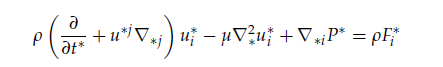
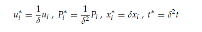
where ρ is constant density, μ is dynamic viscosity ,, are the body forces on the fluid. In some cases, it may be elected to reparametrize the components of the velocity vector, and pressure to
,coordinates xi and time t according to the following form utilizing the non-dimensional quantity d(assumed negative):
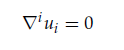
The continuity equation in Cartesian co-ordinates, is
2.1. Data
Eq.(1), together with Eq.(3) and using the initial condition of such that
encompass the NSEs along with an incompressible initial condition. Ensuring periodic boundary 44 conditions specified in [1] defined on a cube domain Ω in
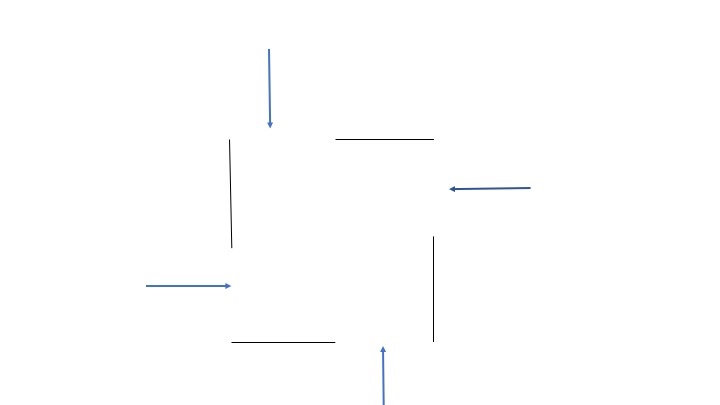
Figure 1. Vortex generation in a 2-D projection of cube.
3. Application
Using Eq.2 above, multiplying the first two components of scale invariant Eq.1 by Cartesian unit vectors respectively and adding modified equations within the set Eq.1 give the following equations, for the resulting composite vector
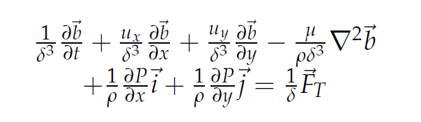
Multiplying Eq. 4 by δ3 and by and, the
component of Eq.1 by δ3 and by
,(again using Eq.2), the addition of the resulting equations [12][13][14] recalling the product rule, produces a form as displayed below in Eq.5, where
. The nonlinear inertial term when added to
and factoring out
gives,
. Here
is a dyadic.
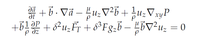
Multiplying Eq.5 by and adding to it
gives:
At this point the z component of the external force, Fz, is assumed to vanish, In this paper Eq.6 is solved, instead of Eq.5. For the ε–periodic solution, it is proposed that integration of divergence or curl of Eq.6 over an arbitrary small volume is equivalent to integration of divergence or curl of Eq.5 for the same volume. That is the extra term’s divergence or curl in Eq.6 when integrated is negligible on set of measure zero. A necessary condition that the form of Eq. 5, call it L1 = 0, is that both the divergence and curl of L1 be zero and upon integrating over a volume U, we introduce a function of t which we call Cs(t).The same is true for the non ε–periodic case where the justification of using Eq 6 instead of 5 will be based on the periodicity of the flow on an interval in has an integral of it’s divergence equal to zero. Proof is straightforward upon taking the divergence and integrating. Next for the curl of the same term and integrating over the same volume we use the fact that
This contribution is also zero due to periodicity of velocities on interval.
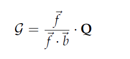
Theorem 3.0.1. Reduced structure form of 3-D Navier-Stokes Equations
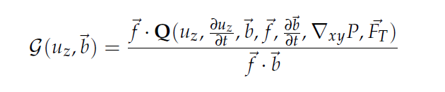
The 3-D Incompressible Navier Stokes equations can be reduced to a simple form as,
where is the nonlinear partial differential operator given by Eq.13, Q is the two dimensional Navier-Stokes operator acting on the vector
defined in the brackets of Eq.17 and
. The terms Ωi contained in
are defined after Eq.10 and are part of the proof of present Theorem 3.0.1.
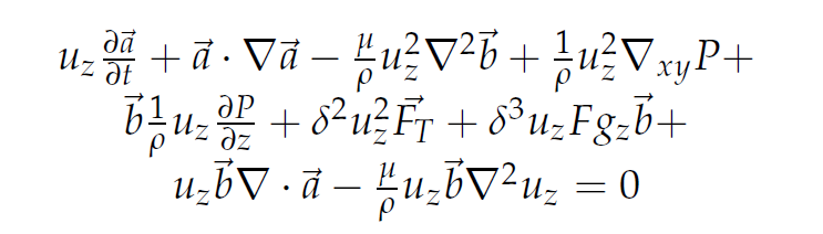
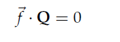
Proof. Taking the geometric product with the inertial vector term in the previous equation Eq.6 given by , it can be shown that in the context of Geometric Algebra [12][14], the following scalar and vector grade equations arise:
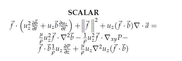
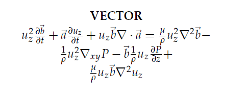
Taking the divergence of the vector equation Eq.8, recalling the product rule, and defining the new term (After taking divergence multiply new equation by H), results in an expression which may be combined with the usage of the scalar equation Eq.7 to produce:

Continuing with the previous paragraph we use the common term appearing in Eq.7,and in the new equation where we took divergence of Eq.8 and multiplied by H. This term in Eq.8 is
. Upon a division of the preceding equation 9 by
, it can be seen to result in the general form:

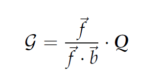
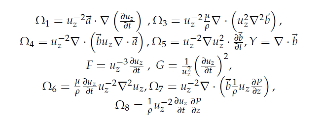
where for brevity, the following symbols have been defined:
It can be seen that the expression beginning with parentheses may be abbreviated into a nonlinear
vector operator Q and so Eq.10 can be written compactly as:
where is the non-linear operator associated with remaining part of Eq.10. Utilizing the continuity
Eq.3, it can be seen that the operator is given by the following expression:

The nonlinear operator form of the NSEs presented is:
This completes the proof.
An important observation is that in Eq.12,

Equation 13 displays a general form which may be expanded and analyzed by allowing a geometric assumption to be undergone, or the general case may also be considered.
4. Two Cases
4.1. The Geometric Case
As a special case, one may consider the case where:
This condition means that the Lie Product of the velocity inertia is entirely perpendicular to the Force terms, and thus refers to a vortex fluid scenario. This condition automatically implies = 0 and so,
4.2. The General Case
For Q, the expressions with and it’s derivative with respect to t factor out completely from the expression and the operator acting on the vector
(that is Eq.4), remains which is identically zero, This means that
may be assumed to be:
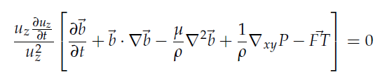
The expression in brackets in Eq.17, for, is the 2-D "plane-parallel" Navier-Stokes Equations and it is well known that if all data of problem are independent of one of x, y, z, then the BVP in Eqs.1, Eqs.3, has a unique solution for all instants of time with no restrictions on smallness of
,
or the domain Ω.[6].
Using Green’s identity, for divergence (see Appendix B), also known as Ostogradsky’s Theorem, it is known that for an arbitrary vector field and scalar field ψ, the following identity holds:
(18)
Eq.16 can be expressed due to integration on a general rectangular volume U as:

Note that the surface integral in Eq.18 is zero since it is taken over six faces of a general rectangular volume, and is a periodic vector field with normals pointing in opposite directions on opposite sides. Here
which is assumed to be equal on the four vertical faces of cube and not equal between the top and bottom face. Also Ω1 is zero using Eq.18 and continuity Eq.3, Ω3 vanishes using Eq.18 as well due to periodic boundary conditions on the cube’s surface. The pressure is expressed using the divergence theorem as a surface integral over the surface. In addition Ω4 and Ω7 vanish using the divergence theorem and the fact that
is periodic on the surface of U.
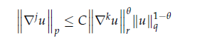
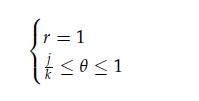
Lemma 1 (Maximum Principle For Eq.19). In this lemma we prove a maximum principle for Eq.19 in the general case where there are no restrictions on Φ and the most general Gagliardo [15]-Nirenberg [16] inequality (see also [17]) is used in this lemma and can be stated as follows, Let 
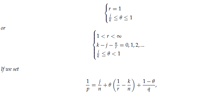
then there exists a constant C independent of u such that ,
Proof. Using the z momentum equation again and multiplying by , for the case,
we obtain for j = 1, k = 2,
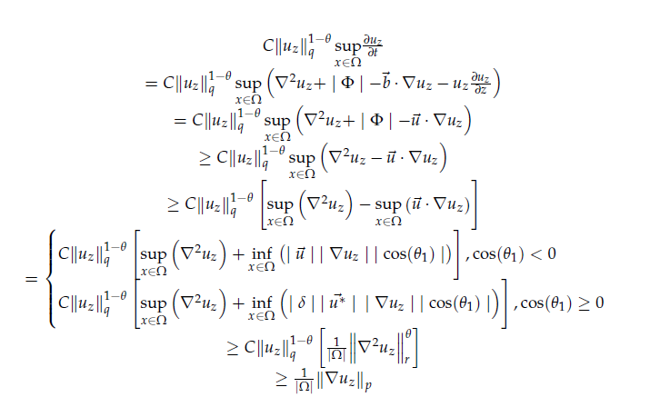
where in the last two lines of 21, the Gagliardo-Nirenberg [15],[16] inequality, Eq 20, has been used, Eq.2 has been used to express in terms of
using the negative term δ, and for
the equality
(A) is used and for
. We abbreviate to the following expression involving the pressure and velocity terms,
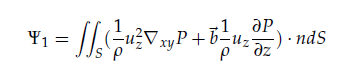
Next it is easy to show using 14, 19 and 21 that,

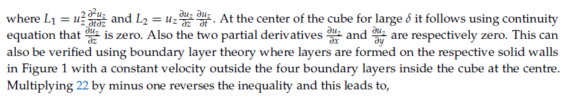

(Note: General case of constant in space but not in time velocity at centre of cube is considered; Also the Poincare inequality has been used. We have used a result which states if the infinity norm is bounded then all the derivatives are bounded.)
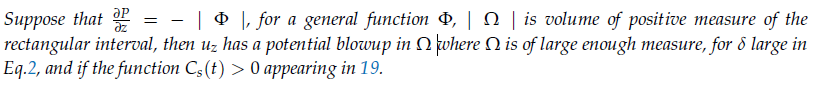
The gradient of pressure is negative inorder to drive the flow, so that -. The determining factor is the integration function in t term
, which is positive and leads to a blowup. To show this the remaining steps are to use the condition,

in Eq. 19. Hence it is shown that,

where B1 is the infimum of F(x, y, z) in the cube which is non-zero since there is a maximum negative flow in the z direction at the centre ( There exists a negative pressure gradient in z driving the flow downwards in cube with vortex in x, y directions ) and . Solving for
in previous equation and differentiating with respect to z the form of the equation results in the following two ordinary differential equations,
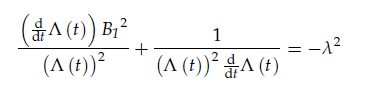
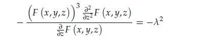
where λ is a separation constant.
References
- C.L. Fefferman Existence and Smoothness of the Navier-Stokes Equation, Millennium Prize Problems, Clay.Math.Inst., Cambridge (MA), (2006) ,57-67.
- J. Leray Sur le mouvement d’un liquide visqueux emplissant l’espace, J. Math. Pures Appl., 12, (1933), 1-82.
- J. Leray Sur le mouvement d’un liquide visqueux emplissant l’espace, Acta Math., 63, (1934),193-248.
- J. Leray Essai sur les mouvements plans d’un fluide visqueux que limitent des parois., J. Math. Pures Appl., 13, (1934), 331-418.
- A.A. Kiselev and O.A. Ladyzhenskaya, On the existence and the uniqueness of the solution of the non-stationary problem for an incompressible visous fluid, Izv.Akad.Nauk.USSR, 21, (1957), 655-680.
- O.A. Ladyzhenskaya, The Mathematical Theory of Viscous Incompressible Flow Gordon and Breach, New York, (1969)
- P. Constantin, C. Foias, O.Manley and R. Temam, Connection between the mathematical theory of the Navier-Stokes equations and the conventional theory of turbulence, C. R. Acad. Sc. Paris, 297, (1983), 599-603.
- P. Constantin, C. Foias, O. Manley and R. Temam, Determining modes and fractal dimension of turbulent flows, J. Fluid Mech, 150, (1985), 427 - 440.
- P. Constantin, P. Lax and A. Majda, A simple one-dimensional model for the three-dimensional vorticity equation, Comm. Pure Appl. Math., 38, (1985), 715 - 724.
- Jens Lorenz and Paulo R. Zingano, Properties at potential blow-up times for the incompressible Navier-Stokes equations, Bol. Soc. Paran. Mat., (3s.) v. 35 2 (2017): 127-158, doi:10.5269/bspm.v35i2.27508.
- C. E. Kyritsis, On the 4th Clay millennium problem: Proof of the regularity of the solutions of the Euler and Navier-Stokes equations, based on the conservation of particles, J. Sci. Res. St., 4, (2017), 304-317.
- T.E. Moschandreou, A Method of Solving Compressible Navier Stokes Equations in Cylindrical Coordinates Using Geometric Algebra,Mathematics (2019), 7(2), 126; https://doi.org/10.3390/math7020126 - 27 Jan 2019.
- T.E. Moschandreou, K.C. Afas Compressible Navier-Stokes Equations in Cylindrical Passages and General Dynamics of Surfaces—(I)-Flow Structures and (II)-Analyzing Biomembranes under Static and Dynamic ConditionsMathematics (2019), 7(11), 1060; https://doi.org/10.3390/math7111060 - 05 Nov 2019.
- T.E. Moschandreou A New Analytical Procedure to Solve Two Phase Flow in Tubes, Math. Comput. Appl. (2018), 23(2), 26; https://doi.org/10.3390/mca23020026 - 23 May 2018
- E. Gagliardo Ulteriori proprietà di alcune classi di funzioni in più variabili,Ricerche Mat., (1959), 8:24–51.
- L.Nirenberg On elliptic partial differential equations. Ann. Scuola Norm. Sup. Pisa (3), (1959), 13:115–162
- A. Fiorenza,M.R. Formica, T. Roskovec and F. Soudský Detailed proof of classical Gagliardo-Nirenberg Interpolation inequality with historical remarks, (2018), arXiv:1812.04281v1 [math. FA]

