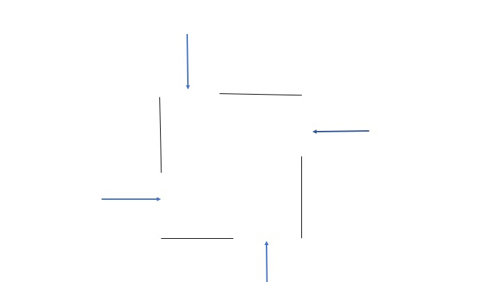
A closely related problem to The Clay Math Institute "Navier-Stokes, breakdown of smooth solutions here on any cube subset of three dimensional space with periodic boundary conditions is examined. The incompressible Navier-Stokes Equations are presented in a new and conventionally different way here, by reducing them to an operator form which is then further analyzed. It is shown that a reduction to a general 2D N-S system decoupled from a 1D non-linear partial differential equation is possible to obtain. This is executed using integration over n-dimensional compact intervals which allows decoupling. Here we extract the measure-zero points in the domain where singularities may occur and are left with a pde that exhibits finite time singularity. The operator form is considered in a physical geometric vorticity case, and a more general case. In the general case, the solution is revealed to have smooth solutions which exhibit finite-time blowup on a fine measure zero set and using the Gagliardo-Nirenberg inequalities it is shown that for any non zero measure set in the form of cube subset of 3D there is finite time blowup. Figure 1 shows the geometry of the problem.
- Navier-Stokes
- compressible
- cylindrical
- Hunter-Saxton
- Biomembranes
The question of whether the solutions to the 3-D- Incompressible N-S equations are globally regular or demonstrate finite time blowup has been a long going debate in mathematics and in general the scientific communities. The Millennium problem posed by the Clay Institute \cite{Feff} is asking for a proof of one of the above conjectures. Seminal papers conducted by Jean Leray \cite{Leray1,Leray2,Leray3} proved that there exists a global (in time) weak solution and a local strong solution of the initial value problem when the domain is all of $\mathbb{R}^3$, that is solutions up to some finite $T^*$ on an interval $[0,T^*]$. While specific cases have approached answers in unique cases, the question of whether there is a unique solution for all instants of time, (ie. a global unique solution) is presently open. It has been shown that there exists a unique global solution for the 2D plane-parallel N-S equations\cite{Kiselev,Ladyzhenskaya}. While at first glance, the NSEs appear as a compact set of PDEs, the fascination with these Partial Differential Equations is only increased by the fact that the nonlinearity of the ensuing expanded equations, appear to be connected with notions of highly chaotic turbulence and vorticity\cite{Const1,Const2,Const3,Viswanathan}. Since the announcement of the Millennium Problem, several results have attempted to comment on the existence and uniqueness of the NSEs. One particularly recent result by Kyritsis noted that there existed indications towards establishing a regularity of solutions regarding the Euler Equations and NSEs more generally; this utilized the conservation of particles\cite{Kyr}.In the present work, to the best of the authors' knowledge, the procedure revealed here has not been previously observed in the literature on the question of Incompressible N-S 3-D existence of unique global solutions, except for compressible flows in \cite{Mosch1,Mosch2,Mosch3}. First, a bounded 3-D rectangle or interval in $\mathbb{R}^3$ with boundary conditions that generate a vortex is considered , and an attempt can be made to reduce the 3-D incompressible NSEs to a one component decoupled velocity field solution under scale invariant transformations, with a separable 2-component velocity field solution. For the variable $z$- component, in particular, a form of solution is extracted in the analysis presented using the divergence form of Green's identity, Ostogradsky's theorem.
\( \textrm{The 3D incompressible unsteady Navier-Stokes Equations (NSEs) in Cartesian coordinates may be listed } \)
\( \textrm{below in compactified form for the velocity field $\textbf{u}^*=u^{*i} \vec{\textbf{e}}_i \phantom{.},\phantom{.}u^{*i}=\{u^*_x,u^*_y,u^*_z\}$:} \)
\( \begin{equation} \label{1} \rho\left(\frac{\partial}{\partial t^*}+u^{*j}\nabla_{*j}\right)u^*_{i}-\mu\nabla^2_{*}u^*_{i}+\nabla_{*i}P^*=\rho F^*_i \end{equation} \)
\( \textrm{In some cases, it may be elected to reparametrize the components of the velocity vector, and pressure } \)\( \textrm{ to $\textbf{u}=(u)^i\vec{\textbf{e}}_i$, $\textbf{P}=(P)^i\vec{\textbf{e}}_i$, coordinates $\textbf{x}_i$ and time $t$} \) \( \textrm{according to the following form utilizing the non-dimensional quantity $\delta$} \).
\( \begin{equation} \label{2} u^*_{i}=\frac{1}{\delta}u_i\phantom{.},\phantom{.}P^*_{i}=\frac{1}{\delta^2}P_i\phantom{.},\phantom{.}x^*_{i}=\delta x_i\phantom{.},\phantom{.}t^*=\delta^2t \end{equation} \)
\( \textrm{The continuity equation in Cartesian co-ordinates, is } \begin{equation} \label{3} \nabla^{i}u_i=0 \end{equation} \).
The flow boundary consists of a cube in \( R^3 \) and the following projection flow onto the plane is used.
\( \textrm{Using the above, multiplying the first two components of scale invariant Eq.1 by Cartesian unit vectors} \)
\( \textrm{$\vec{i}=(1,0,0)$, $ \vec{j}=(0,1,0)$ respectively and adding modified equations within the set Eq. 1} \)
\( \textrm{give the following equations, for the resulting composite vector $\vec{b}= \frac{1}{\delta} u_x \vec{i}+\frac{1}{\delta} u_y\vec{j}$} \) .
3)


the addition of the resulting equations,


5)

6)


