Multi-Granularity Process Analytics

Version	Summary	Created by	Modification	Content Size	Created at	Operation
1		Marco Reis	+ 1737 word(s)	1737	2021-11-18 07:29:28	\|
2	Done	Jason Zhu	Meta information modification	1737	2021-12-22 02:23:51	\|

This entry is adapted from the peer-reviewed paper 10.3390/pr7020061

Data can be aggregated to lower resolution representations according to a certain rational or optimality criterion in a certain pre-defined sense. In this situation, partial information from all observations is retained and at the same time the amount of data analysed is greatly reduced. The level of resolution or granularity adopted may be different for each variable under analysis. Methods for dealing with these data structures are called multiresolution or multi-granularity, and are newcomers to the Process Analytical toolkit.

Multi-Granularity data aggregation industrial big data multiresolution temporal aggregation

1. Multi-Granularity Methods

Multi-granularity methods (also called multiresolution methods) address the challenge of handling the coexistence of data with different granularities or levels of aggregation, i.e., with different resolutions (not to be confounded with the Metrology concept with the same name). Therefore, they are primarily a response to the demand imposed by modern data acquisition technologies that create multi-granularity data structures in order to keep up with the data flood—data is being aggregated in summary statistics or features, instead of storing every collected observation. But, as will be explored below, multi-granularity methods can also be applied to improve the quality of the analysis, even when raw data are all at the same resolution. By selectively introducing granularity in each variable (if necessary), it is possible to optimize and significantly improve the performance of, for instance, predictive models.

The usual tacit assumption for data analysis is that all available records have the same resolution or granularity, usually considered to be concentrated around the sampling instants (which should, furthermore, be equally spaced). Analyzing modern process databases, one can easily verify that this assumption is frequently not met. It is rather common to have data collectors taking data from the process pointwisely; i.e., instantaneously, at a certain rate, while quality variables often result from compound sampling procedures, i.e., material is collected during some predefined time, after which the resulting volume is mixed and submitted to analysis; the final value represents a low resolution measurement of the quality attribute with a time granularity corresponding to the material collection period. Still other variables can be stored as averages over hours, shifts, customer orders, or production batches, resulting from numerical operations implemented in the process Distributed Control Systems (DCS) or by operators. Therefore, modern databases present, in general, a Multiresolution data structure, and this situation will tend to be found with increasing incidence as Industry 4.0 takes its course.

Multiresolution structures require the use of dedicated modelling and processing tools that effectively deal with the multiresolution character and optimally merge multiple sources of information with different granularities. However, this problem has been greatly overlooked in the literature. Below, researchers refer to some of the efforts undertaken to explicitly incorporate the multiresolution structure of data in the analysis or, alternatively (but also highly relevant and opportune), to take advantage of introducing it (even if it is no there initially), for optimizing the analysis performance.

2. Multi-Granularity Methods for Process Monitoring

An example, perhaps isolated, of a process monitoring approach developed for handling simultaneously the complex multivariate and multiscale nature of systems and the existence of multiresolution data collected from them, was proposed by Reis and Saraiva ^[1]: MR-MSSPC. Similarly to MSSPC ^[2]^[3], this methodology implements scale-dependent multivariate statistical process control charts on the wavelet coefficients (fault detection and feature extraction stage), followed by a second confirmatory stage that is triggered if any event is detected at some scale during the first stage. However, the composition of the multivariate models available at each scale depends on the granularity of data collected and is not the same for all of them, as happened in MSSPC. This implies algorithmic differences in the two stages as well as on the receding horizon windows used to implement the method online. This results in a clearer definition of the regions where abnormal events take place and a more sensitive response when the process is brought back to normal operation. MR-MSSPC brings out the importance of distinguishing between multiresolution (multi-granularity) and multiscale concepts: MSSPC is a multiscale, single-resolution approach, whereas MR-MSSPC is a multiscale, multiresolution methodology.

3. Multi-Granularity Modelling and Optimal Estimation

Willsky et al. developed, in a series of works, the theory for Multiresolution Markov models, which could then be applied to signal and image processing applications ^[4]^[5]^[6]. This class of models share a similar structure to the classical state-space formulation, but they are defined over the scale domain, rather than the time domain. These allow data analyses over multiple resolutions (granularity levels), which is the fundamental requirement for implementing optimal fusion schemes for images with different resolutions such as satellite and ground images. In this regard, Multiresolution Markov models were developed for addressing multiresolution problems in space (e.g., image fusion). However, they do not apply when the granularity concerns time. In this case, new model structures are required that should be flexible enough to accommodate for measurements with different granularities. In the scope of multiresolution soft sensors (MR-SS) for industrial applications, Rato and Reis ^[7] proposed a scalable model structure with such multi-granularity capability embedded—the scalability arises from its estimability in the presence of many variables, eventually highly correlated (a feature inherited from Partial Least Squares, PLS, which is estimation principle adopted). The use of a model structure (MR-SS) that is fully consistent with the multiresolution data structure leads to: (i) an increase in model interpretability (the modelling elements regarding multiresolution and dynamic aspects are clearly identified and accommodated); (ii) higher prediction power (due to the use of more parsimonious and accurate models); (iii) paves the way to the development of advanced signal processing tools; namely, optimal multiresolution Kalman filters ^[8]^[6]^[9]^[10].

But there is another motivation for being interested in multiresolution analysis besides the need to handle it when present in data—even when the data is available at a single-resolution (i.e., all variables have the same granularity), there is no guarantee whatsoever that this native resolution is the most appropriate for analysis. On the contrary, there are reasons to believe the opposite, as this choice is usually made during the commissioning of the IT infrastructure, long before engineers or data analysts (or even someone connected to the operation or management of the process) become involved in the development of data-driven models. Therefore, it should be in the best interest of the analyst to have the capability of tuning the optimal granularity to use for each variable, in order to maximize the quality of the outputs of data analysis. The optimal selection of variables’ resolution or granularity has been implemented with significant success for developing inferential models for quality attributes in both batch ^[11] as well as continuous processes ^[12]. Notably, it can be theoretically guaranteed that the derived multiresolution models perform at least as well as their conventional single-resolution counterparts. For the sake of illustration, in a case study with real data, the improvement in predictive performance achieved was of 54% ^[11]. Figure 1 presents a scheme highlighting the set of variables selected in this case study, to estimate the target response (polymer viscosity) and the associated optimal resolution at which they should be represented.

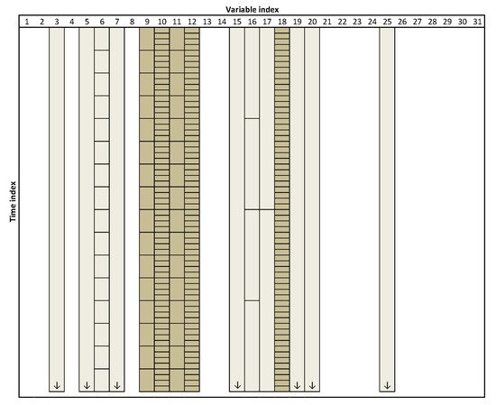
Figure 1. Schematic representation of the variables/resolutions selected for building the model. The size of the boxes represent the adopted granularity for each variable; the lighter shades indicate variable/resolutions that were pre-selected by the algorithm but discarded afterwards; the final combination of variables/resolution used in the model are represented with a darker color).

4. Multiresolution Projection Frameworks for Industrial Data

The computation of approximations at different resolutions can be done in a variety of ways. Using wavelet-based frameworks is one of them, but the resulting approximation sequence present granularities following a dyadic progression, i.e., where the degree of delocalization doubles when moving from one resolution level to the next. But the time-granularity may also be flexibly imposed by the user, according to the nature of the task or decision to be made. In this case, one must abandon the classic wavelet-based framework, and work on averaging operators that essentially perform the same actions on the raw signals as wavelet approximation (or low-pass) filters do. These averaging operations can also be interpreted as projections to approximation subspaces, as in the wavelet multiresolution construct, but now these subspaces are more flexibly obtained and do not have to conform to the rigid structure imposed in the wavelet framework.

One problem multiresolution frameworks have to deal with when processing industrial data, is missing data. This is an aspect that wavelet multiresolution projections cannot handle by default, and the same applies to conventional averaging operators. One solution found to this prevalent problem (all industrial databases have many instances of missing data, with different patterns and origins) can be found in the scope of uncertainty-based projection methods ^[13]. In this setting, each data record is represented by a value and the associated uncertainty. Values correspond to measurements, whereas the uncertainty is a “parameter, associated with the result of a measurement, that characterizes the dispersion of the values that could reasonably be attributed to the measurand” ^[14]. According to the “Guide to the Expression of Uncertainty in Measurement” (GUM) the standard uncertainty, U(Xi)(to which researchers will refer here simply as uncertainty), is expressed in terms of a standard deviation of the values collected from a series of observations (the so called Type A evaluation), or through other adequate means (Type B evaluation), namely, relying upon an assumed probability density function expressing a degree of belief. With the development of sensors and metrology, both quantities are now routinely available and their simultaneous use is actively promoted and even enforced by standardization organizations. Classical data analysis tasks, formerly based strictly on raw data, such as Principal Components Analysis and Multivariate Linear Regression approaches (e.g., Ordinary Least Squares, Principal Components Regression) are also being upgraded to their uncertainty-based counterparts, that explicitly consider combined data/uncertainty structures ^[15]^[16]^[17]^[18]^[19]^[20]. The same applies to multiresolution frameworks where the averaging operator may incorporate both aspects of data (measurements and their uncertainty), and, in this way directly address and solve, in an elegant way, the missing data problem: a missing value can be easily replaced by an estimate of it together the associated uncertainty. In the worst case, the historical mean can be imputed, having associated the historical standard deviation, but often more accurate missing data imputation methods can be adopted to perform this task ^[21]^[22]^[23]^[24]. Examples of multiresolution projection frameworks developed for handling missing data and heteroscedastic uncertainties in industrial settings can be found in ^[13].

References

Reis, M.S.; Saraiva, P.M. Multiscale Statistical Process Control with Multiresolution Data. AICHE J. 2006, 52, 2107–2119.
Bakshi, B.R. Multiscale PCA with Application to Multivariate Statistical Process Control. AICHE J. 1998, 44, 1596–1610.
Reis, M.S.; Bakshi, B.R.; Saraiva, P.M. Multiscale statistical process control using wavelet packets. AICHE J. 2008, 54, 2366–2378.
Bassevile, M.; Benveniste, A.; Willsky, A.S. Multiscale Autoregressive Processes, Part I: Schur-Levinson Parametrizations. IEEE Trans. Signal Process. 1992, 40, 1915–1934.
Bassevile, M.; Benveniste, A.; Willsky, A.S. Multiscale Autoregressive Processes, Part II: Lattice Structures for Whitening and Modeling. IEEE Trans. Signal Process. 1992, 40, 1935–1954.
Willsky, A.S. Multiresolution Markov Models for Signal and Image Processing. Proc. IEEE 2002, 90, 1396–1458.
Rato, T.J.; Reis, M.S. Multiresolution Soft Sensors (MR-SS): A New Class of Model Structures for Handling Multiresolution Data. Ind. Eng. Chem. Res. 2017, 56, 3640–3654.
Bassevile, M.; Benveniste, A.; Chou, K.C.; Golden, S.A.; Nikoukhah, R.; Willsky, A.S. Modeling and Estimation of Multiresolution Stochastic Processes. IEEE Trans. Inf. Theory 1992, 38, 766–784.
Chou, K.C.; Willsky, A.S.; Benveniste, A. Multiscale Recursive Estimation, Data Fusion, and Regularization. IEEE Trans. Autom. Control 1994, 39, 464–478.
Chou, K.C.; Willsky, A.S.; Nikoukhah, R. Multiscale Systems, Kalman Filters, and Riccati Equations. IEEE Trans. Autom. Control 1994, 39, 479–492.
Geert, G.; Van Impe, J.F.M.; Reis, M.S. Finding the optimal time resolution for batch-end quality prediction: MRQP—A framework for Multi-Resolution Quality Prediction. Chemom. Intell. Lab. Syst. 2018, 172, 150–158.
Rato, T.J.; Reis, M.S. Building Optimal Multiresolution Soft Sensors for Continuous Processes. Ind. Eng. Chem. Res. 2018, 57, 9750–9765.
Reis, M.S.; Saraiva, P.M. Generalized Multiresolution Decomposition Frameworks for the Analysis of Industrial Data with Uncertainty and Missing Values. Ind. Eng. Chem. Res. 2006, 45, 6330–6338.
BIPM; IEC; IFCC; ISO; IUPAC; IUPAP; OIML. Guide to the Expression of Uncertainty; ISO: Geneva, Switzerland, 1993.
Bro, R.; Sidiropoulos, N.D.; Smilde, A.K. Maximum Likelihood Fitting Using Ordinary Least Squares Algorithms. J. Chemom. 2002, 16, 387–400.
Reis, M.S.; Saraiva, P.M. Integration of Data Uncertainty in Linear Regression and Process Optimization. AICHE J. 2005, 51, 3007–3019.
Río, F.J.; Rio, J.; Rius, F.X. Prediction Intervals in Linear Regression Taking into Account Errors in Both Axis. J. Chemom. 2001, 15, 773–788.
Wentzell, P.D.; Andrews, D.T.; Hamilton, D.C.; Faber, K.; Kowalski, B.R. Maximum Likelihood Principal Component Analysis. J. Chemom. 1997, 11, 339–366.
Wentzell, P.D.; Andrews, D.T.; Kowalski, B.R. Maximum Likelihood Multivariate Calibration. Anal. Chem. 1997, 69, 2299–2311.
Wentzell, P.D.; Lohnes, M.T. Maximum Likelihood Principal Component Analysis with Correlated Measurements Errors: Theoretical and Practical Considerations. Chemom. Intell. Lab. Syst. 1999, 45, 65–85.
Arteaga, F.; Ferrer, A. Dealing with Missing Data in MSPC: Several Methods, Different Interpretations, Some Examples. J. Chemom. 2002, 16, 408–418.
Little, R.J.A.; Rubin, D.B. Statistical Analysis with Missing Data, 2nd ed.; Wiley: Hoboken, NJ, USA, 2002.
Nelson, P.R.C.; Taylor, P.A.; MacGregor, J.F. Missing Data Methods in PCA and PLS: Score Calculations with Incomplete Observations. Chemom. Intell. Lab. Syst. 1996, 35, 45–65.
Walczak, B.; Massart, D.L. Dealing with Missing Data. Chemom. Intell. Lab. Syst. 2001, 58, 15–27, 29–42.

© Text is available under the terms and conditions of the Creative Commons Attribution (CC BY) license; additional terms may apply. By using this site, you agree to the Terms and Conditions and Privacy Policy.

Upload a video for this entry

Information

Subjects: Engineering, Chemical; Computer Science, Artificial Intelligence; Engineering, Industrial

Contributor MDPI registered users' name will be linked to their SciProfiles pages. To register with us, please refer to https://encyclopedia.pub/register :

Marco Reis

View Times: 445

Update Date: 22 Dec 2021

Table of Contents

Video Upload Options

Confirm