Multiphysics Data for Mineral Exploration

Version	Summary	Created by	Modification	Content Size	Created at	Operation
1		Michael S. Zhdanov	+ 1620 word(s)	1620	2021-07-10 08:21:30	\|
2	The format is correct	Lindsay Dong	Meta information modification	1620	2021-07-12 03:28:58	\|

This entry is adapted from the peer-reviewed paper 10.3390/geosciences11060262

Different geophysical methods provide information about various physical properties of rock formations and mineralization. In many cases, this information is mutually complementary. At the same time, inversion of the data for a particular survey is subject to considerable uncertainty and ambiguity as to causative body geometry and intrinsic physical property contrast. One productive approach to reducing uncertainty is to jointly invert several types of data. Non-uniqueness can also be reduced by incorporating additional information derived from available geological and/or geophysical data in the survey area to reduce the searching space for the solution. This additional information can be incorporated in the form of a joint inversion of multiphysics data.

joint inversion multiphysics three-dimensional Gramian constraints focusing constraints

1. Introduction

Information from different surveys is mutually complementary, which makes it natural to consider a joint inversion of the data to a shared model, a process which can be implemented using several different physical and mathematical approaches. Integration of multiphysics data also helps reduce ambiguity, which is typical for geophysical inversions. Over the last decades, several approaches were introduced to joint inversion of geophysical data. The traditional technique is based on using the known petrophysical relationships between different physical properties of the rocks within the framework of the inversion process ^[1]^[2]^[3]^[4]^[5]^[6]^[7]^[8]^[9]. The joint inversion can use these relationships or can indicate and characterize the existence of this correlation, yielding an improved final model.

Another approach to joint inversion uses a clustering concept from statistics, which assumes that the subsurface geology can be described by the models with petrophysical parameters forming a specific number of the known clusters in the space of the models (e.g., ^[10]^[11]^[12]). This approach requires a priori knowledge of the parameters of these clusters, which is related to the lithology of the rocks.

In the cases where the model parameters are not correlated but nevertheless have similar geometrical features, joint inversion can be based on structure-coupled constraints. For example, these constraints can be implemented by the cross-gradient method, which enforces the gradients of the model parameters to be parallel ^[13]^[14]^[15]^[16]^[17].

There still exist many challenges in incorporating typical geological complexity in joint inversion. For example, analytic, empirical, or statistical correlations between different physical properties may exist for only part of the shared earth model, and their specific form may be unknown. Features or structures that are present in the data of one geophysical method may not be present in the data generated by another geophysical method or may not be equally resolvable.

2. Gramian Constraints

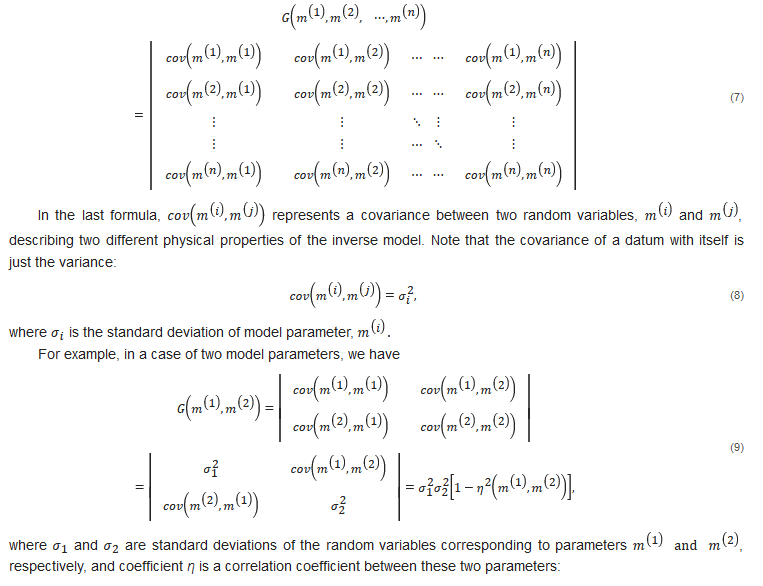
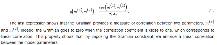
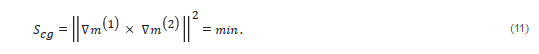
Gramian constraints enforce the correlation between different parameters or their transforms ^[6]^[7]. They are implemented by using a Gramian mathematical operator in regularized inversion, which results in producing multimodal inverse solutions with enhanced correlations between the different model parameters or their attributes.

Let us consider forward geophysical problems for multiple geophysical data sets. These problems can be described by the following operator relationships:

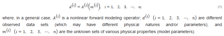
Note that diverse model parameters may have different physical dimensions (e.g., density is measured in g/cm³, resistivity is measured in Ohm-m, etc.). It is convenient to introduce the dimensionless weighted model parameters, m ˜ ( i ) = W m ( i ) m ( i ) , where W m ( i ) is the corresponding linear operator of model weighting ^[7].

Joint inversion of multiphysics data can be reduced to minimization of the following parametric functional,

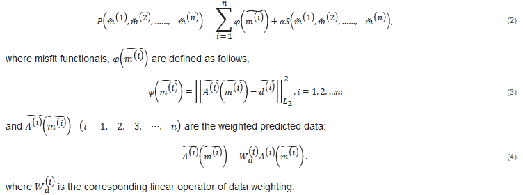
The selection of the model and data weights was discussed in many publications on inversion theory. For example, in the framework of the probabilistic approach ^[18], the weights were determined as inverse data covariance or model covariance matrices. In the framework of the deterministic approach ^[19], the weights were determined as inverse integrated sensitivity matrices.

Gramian provides a measure of correlation between the different model parameters or their attributes. By imposing an additional requirement minimizing the Gramian in regularized inversion, we obtain multimodal inverse solutions with enhanced correlations between the various model parameters.

For example, in the case of two model parameters (e.g., density and magnetic susceptibility), the Gramian is computed as follows:

where (⋅,⋅) stands for the inner product in the corresponding Hilbert space of model parameters ^[7].

In a general case of n model parameters, the Gramian is computed as the determinant of the Gram matrix as follows:

One can also choose various metrics of the Hilbert space in Equation (6), used in the definition of the Gramian ^[7]. This brings additional flexibility to the type of coupling between different model parameters enforced by the Gramian constraints, which is illustrated below.

We can also introduce a Hilbert space with the metric defined by the covariance between random variables, representing different model parameters. Under these assumptions, the Gramian stabilizing functional arises as a determinant of the covariance matrix between different model parameters ^[20]:

We have demonstrated above that Gramian approach is based on the concept of linear correlation; however, by applying this concept to the transforms of the model parameters, we can amplify a variety of different properties in joint inversion. For example, Gramian of the gradients of the model parameters results in structural correlations. Gramian applied to the nonlinear transforms of the model parameters results in nonlinear correlations. Gramian applied locally (in the framework of the localized approach) results in spatially variable relationships between different physical properties. In short, the Gramian approach is not limited to a strict linear correlation assumption. This property of Gramian approach will be illustrated below in the sections dedicated to the structural and localized Gramian-based constraints.

3. Joint Inversion Using Gramian-Based Structural Constraints

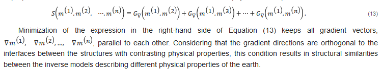
One of the most widely used approaches to imposing the structural constraints on the results of the joint inversion is based on the method of cross gradients ^[13]^[14]^[15]^[16]^[17]. The basic idea behind this method is that the gradients of the model parameters should be parallel in order to enforce the geometrical similarities between the interfaces of the models. Within the framework of the cross-gradient method, this requirement can be achieved by minimizing the norm square of the cross product of the gradients of these functions:

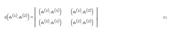
In the framework of the Gramian approach, the same requirement for the gradients of the model parameters being parallel is achieved by minimizing the structural Gramian functional, G ∇ , which, in a case of two physical properties, can be written using matrix notations, as follows:

By minimizing the Gramian functional, G ∇ , we enforce the linear correlation between the gradients of the model parameters, making these vectors parallel to each other. The method can also be naturally expanded for any number, n, of the model parameters, by considering the corresponding Gramian matrices between the gradients of the different parameters. The practical advantage is, again, in the quadratic nature of this functional, which was demonstrated in ^[6]^[7]. This property was proved based on the concept of the Gramian space which was shown to be a Hilbert space with all related useful properties.

For example, we can introduce a stabilizing term in the parametric functional shown in Equation (2) as a superposition of the structural Gramians between the first and all other physical model parameters:

4. Localized Gramian Constraints

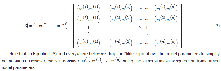
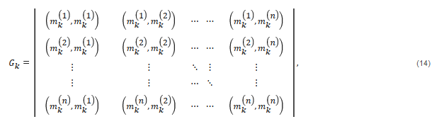
The constraints based on minimization of the Gramian of the model parameters, Equations (5) and (6), or of their gradients, Equations (12) and (13), can be treated as the global constraints, because they enforce similar correlation conditions over the entire inversion domain. In practical applications, however, the specific form of the correlations may vary within the area of investigation. To address this situation, we can subdivide the inversion domain, D, into N subdomains, D k , with potentially different types of relationships between the different model parameters, and define the Gramians, G k , for each of these subdomains separately:

In this case, the localized Gramian constraints will be based on using the following stabilizing functional:

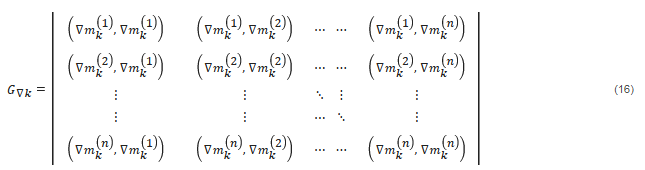
In a similar way, we can introduce localized Gramian-based structural constraints, using the localized Gramian of model parameter gradients, G ∇ k , defined by the following formula:

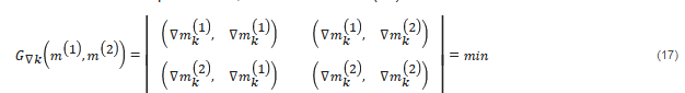
For example, in a case of two model parameters, localized Gramian (16) takes the form:

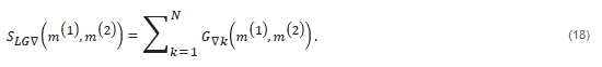
and the corresponding stabilizing functional is written as follows:

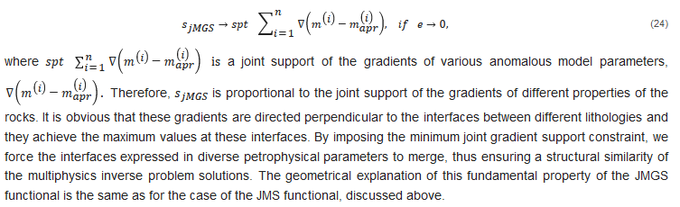
5. Joint Focusing Constraints

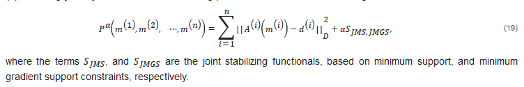
The structural similarities between various petrophysical models of the subsurface can be enforced by using the joint total variation or focusing stabilizers ^[21]^[22]. For the solution of a nonlinear inverse problem shown in Equation (1), following ^[21]^[22], we introduce the following parametric functional with focusing stabilizers,

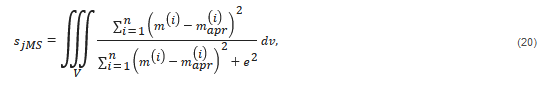
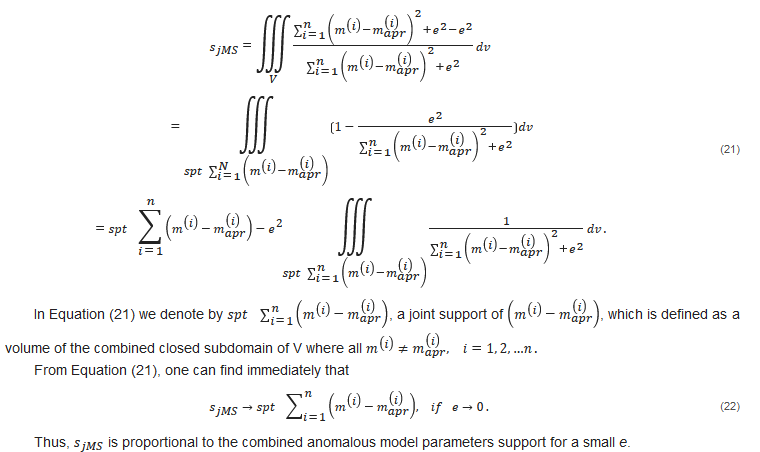
The joint minimum support stabilizer,

is proportional to the combined volume, or support, occupied by domains with anomalous physical parameters for small e.

Indeed, we can rewrite Equation (20) as follows:

It can be easily established by a simple geometrical analysis that the combined anomalous model parameters support reaches the minimum when the volumes occupied by anomalous domains representing various physical properties coincide. Indeed, if the anomalous properties are in different locations, their combined support is larger in comparison to cases when the locations are the same.

A joint minimum gradient support functional (JMGS) is defined as follows:

Repeating the algebraic transformation presented in expression (21), one can demonstrate that:

The minimization of the parametric functional shown in Equation (19) is based on the re-weighted regularized conjugate gradient method (RRCG) ^[7], which iteratively updates the model parameters to minimize the parametric functional and the misfit between the observed and predicted data. The inversion iterates until the misfit reaches a given threshold.

6. Conclusions

Interpretation of multimodal geophysical data represents a data fusion problem, as different geophysical fields provide information about different physical properties of the Earth. In many cases, various geophysical data are complementary, making it natural to consider their joint inversion based on correlations between the different physical properties of the rocks. By using Gramian or joint focusing constraints, we are able to invert jointly multimodal geophysical data by enforcing the correlations or shape similarities between the different model parameters or their attributes. The case studies for joint inversion of various geophysical data demonstrate that the joint inversion enhances the produced subsurface images of the geological target.

References

Afnimar, A.; Koketsu, K.; Nakagawa, K. Joint inversion of refraction and gravity data for the three-dimensional topography of a sediment–basement interface. Geophys. J. Int. 2002, 151, 243–254.
Hoversten, G.M.; Cassassuce, F.; Gasperikova, E.; Newman, G.A.; Chen, J.; Rubin, Y.; Hou, Z.; Vasco, D. Direct reservoir parameter estimation using joint inversion of marine seismic AVA and CSEM data. Geophysics 2006, 71, C1–C13.
Moorkamp, M.; Heincke, B.; Jegen, M.; Robert, A.W.; Hobbs, R.W. A framework for 3-D joint inversion of MT, gravity and seismic refraction data. Geophys. J. Int. 2011, 184, 477–493.
Moorkamp, M.; Lelièvre, P.; Linde, N.; Khan, A. Integrated Imaging of the Earth: Theory and Applications; Geophysical Monograph Series; Wiley: Hoboken, NJ, USA, 2016.
Gao, G.; Abubakar, A.; Habashy, T.M. Joint petrophysical inversion of electromagnetic and full-waveform seismic data. Geophysics 2012, 77, WA3–WA18.
Zhdanov, M.S.; Gribenko, A.V.; Wilson, G. Generalized joint inversion of multimodal geophysical data using Gramian constraints. Geophys. Res. Lett. 2012, 39, L09301.
Zhdanov, M.S. Inverse Theory and Applications in Geophysics; Elsevier: Amsterdam, The Netherlands, 2015.
Giraud, J.; Pakyuz-Charrier, E.; Jessell, M.; Lindsay, M.; Martin, R.; Ogarko, V. Uncertainty reduction through geologically conditioned petrophysical constraints in joint inversion. Geophysics 2017, 82, ID19–ID34.
Giraud, J.; Ogarko, V.; Lindsay, M.; Pakyuz-Charrier, E.; Jessell, M.; Martin, R. Sensitivity of constrained joint inversions to geological and petrophysical input data uncertainties with posterior geological analysis. Geophys. J. Int. 2019, 218, 666–688.
Lelièvre, P.G.; Farquharson, C.G.; Hurich, C.A. Joint inversion of seismic traveltimes and gravity data on unstructured grids with application to mineral exploration. Geophysics 2012, 77, K1–K15.
Sun, J.; Li, Y. Joint inversion of multiple geophysical data using guided fuzzy c-means clustering. Geophysics 2016, 81, ID37–ID57.
Sun, J.; Li, Y. Joint inversion of multiple geophysical and petrophysical data using generalized fuzzy clustering algorithms. Geophys. J. Int. 2017, 208, 1201–1216.
Gallardo, L.A.; Meju, M.A. Characterization of heterogeneous near-surface materials by joint 2D inversion of DC resistivity and seismic data. Geophys. Res. Lett. 2003, 30, 1658.
Gallardo, L.A.; Meju, M.A. Joint two-dimensional DC resistivity and seismic travel-time inversion with cross-gradients constraints. J. Geophys. Res. 2004, 109, B03311.
Gallardo, L.A.; Meju, M.A. Joint two-dimensional cross-gradient imaging of magnetotelluric and seismic traveltime data for structural and lithological classification. Geophys. J. Int. 2007, 169, 1261–1272.
Gallardo, L.A.; Meju, M.A. Structure-coupled multi-physics imaging in geophysical sciences. Rev. Geophys. 2011, 49, RG1003.
Hu, W.Y.; Abubakar, A.; Habashy, T.M. Joint electromagnetic and seismic inversion using structural constraints. Geophysics 2009, 74, R99–R109.
Tarantola, A. Inverse Problem Theory; Elsevier: Amsterdam, The Netherlands, 1987.
Zhdanov, M.S. Geophysical Inverse Theory and Regularization Problems; Elsevier: Amsterdam, The Netherlands, 2002.
Shraibman, V.I.; Zhdanov, M.S.; Vitvitsky, O.V. Correlation methods of transformation and interpretation of geophysical anomalies. Geophys. Prospect. 1980, 28, 919–934.
Molodtsov, D.; Troyan, V. Multiphysics joint inversion through joint sparsity regularization. In Expanded Abstracts, Proceedings of the 88th SEG International Exposition and Annual Meeting, Houston, TX, USA, 29 September 2017; Society of Exploration Geophysicists: Tulsa, OK, USA, 2017; pp. 1262–1267.
Zhdanov, M.S.; Cuma, M. Joint inversion of multimodal data using focusing stabilizers and Gramian constraints. In Expanded Abstracts, Proceedings of the 89th SEG International Exposition and Annual Meeting, Anaheim, CA, USA, 14–19 October 2018; Society of Exploration Geophysicists: Tulsa, OK, USA, 2018; pp. 1430–1434.

© Text is available under the terms and conditions of the Creative Commons Attribution (CC BY) license; additional terms may apply. By using this site, you agree to the Terms and Conditions and Privacy Policy.

Upload a video for this entry

Information

Subjects: Physics, Applied

Contributor MDPI registered users' name will be linked to their SciProfiles pages. To register with us, please refer to https://encyclopedia.pub/register :

Michael Zhdanov

View Times: 408

Update Date: 13 Jul 2021

Table of Contents

Video Upload Options

Confirm