 +1 credit
| Version | Summary | Created by | Modification | Content Size | Created at | Operation |
|---|---|---|---|---|---|---|
| 1 | Renato Morbidelli | + 3121 word(s) | 3121 | 2021-04-25 08:49:23 | | | |
| 2 | Conner Chen | -6 word(s) | 3115 | 2021-04-27 05:15:49 | | | | |
| 3 | Conner Chen | -4 word(s) | 3117 | 2021-04-27 05:17:10 | | | | |
| 4 | Conner Chen | -4 word(s) | 3117 | 2021-04-27 05:17:48 | | |
Video Upload Options
As is widely recognized, rainfall data is necessary for the mathematical modelling of extreme hydrological events, such as droughts or floods, as well as for evaluating surface and subsurface water resources and their quality. The phase, quantity, and elevation of generic hydrometeors in the atmosphere can be estimated by ground-based radars. Satellites can provide images with visible and infrared radiation, and they can also serve as platforms for radiometers to derive the quantity and phase of hydrometeors. Radars and satellites provide spatial information on precipitation at wide scales, avoiding many problems connected to local ground measurements, including those for the areal inhomogeneity of a network. However, direct rainfall observations at point scale can be obtained only by rain gauges installed at the soil surface.
1. Recording of rainfall data
Direct rainfall data can be automatically recorded or not. Typically, non-recording gauges are open receptacles with vertical sides, where the rainfall is derived by human observation on a graduated cylinder. Recording gauges automatically acquire precipitation depths at specified time steps and can be of different types: weighing, float, or tipping bucket gauges. A more recent device is the disdrometer, which can detect the size distribution and speed of falling hydrometeors. A weighing-type rain gauge records the weight of the receiving container and the accumulated rainfall with a spring mechanism or a system of balance weights. A float-type rain gauge consists of a chamber containing a float that rises vertically when the water level increases. A tipping-bucket-type rain gauge works by means of a two-bucket system. The exchanging motion of the tipping buckets generates a signal, corresponding to a rainfall depth equal to the ratio between the water volume that produces a tipping and the surface area of the collector. The signal is recorded, providing a very accurate measure of rainfall depth. In fact, most tipping bucket sensors are set up to obtain one signal for each 0.1 or 0.2 mm of rainfall.
When the direct local rainfall was recorded by means of human observation, a manual transcription of the total depth accumulated, typically in the previous 24 h, was performed. With the spread of automatic recordings, first on paper rolls (e.g., [1]) and later on digital supports, a higher temporal aggregation (or time resolution), ta, of rainfall observation was achieved. Historical series of rainfall data are characterized by different ta, due to the rain gauge type used, adopted recording system, and specific interests of the data owner.
From this historical background, it is clear that until the introduction of digital data loggers, rainfall data were characterized by coarse aggregation time, which may have influenced the results obtained by different kinds of analyses. As an example, several researchers evaluated the effect of coarse time resolution in estimating annual maximum rainfall depths, Hd, with fixed timescales, d [2][3][4][5][6][7][8][9][10][11][12][13]. All these studies showed that for d comparable with ta, the actual values of Hd may be considerably underestimated by up to 50%. Thus, long series of Hd values typically include a relevant number of possible underestimated values deriving from rainfall data with coarse ta, grouped with elements obtained from high-time-resolution data recorded in the last two to three decades. This issue, together with other crucial elements (relocation of stations, use of different rain gauge types, and change of station surroundings), may determine relevant effects on many related investigations, such as those related to the determination of rainfall depth–duration–frequency curves [13] and the evolution of extreme rainfall trends [14].
The problem of underestimated annual maximum rainfall depth could be solved for durations greater than 1 h by adopting one of the methodologies suggested by the scientific literature [2][3][4][5][6][7][8][9][10][11][12][13], while the same cannot be easily done for the analysis of heavy rainfalls characterized by sub-hourly durations. In fact, long Hd series for d < 1 h are rarely available for most geographical areas [14]. The number of rain gauges operative worldwide is approximately in the range 150,000–250,000 [15][16][17][18][19]. As networks of different geographical areas have specific histories and management objectives, the time resolution of the available rainfall data may differ.
The main objective of this review paper is to address the aforementioned issues, regardless of the equally important problem of measurement errors, to improve the use of historical extreme rainfall series through their homogenization with respect to ta. Particular attention is reserved for the correction of Hd series, with the aim of avoiding distortions in climate change detection and hydraulic structures design.
2. Rainfall Data Characteristics
Rainfall data available in several geographic areas are characterized by different temporal aggregation, mainly due to the specific network scope manager and to the technology of the devices used. At present, most rainfall data are continuously recorded in digital data loggers, allowing the adoption of any aggregation time interval, even equal to 1 min (Figure 1).
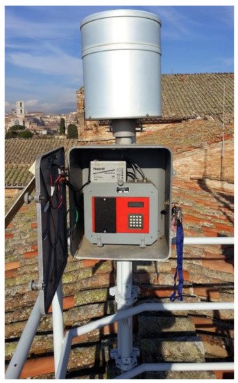
Figure 1. Rain gauge with digital data logger correctly working at Perugia (central Italy).
Until the 1990s, rainfall observations were recorded on paper rolls (see Figure 2) typically with ta = 30 min or 1 h. In addition, before the Second World War, the time resolution of rainfall was daily, with manual recording once a day at a fixed time (see Figure 3).
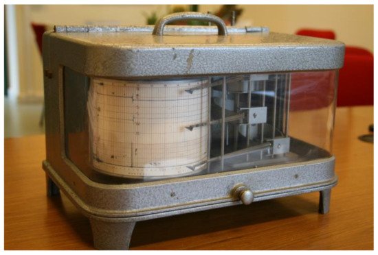
Figure 2. A typical mechanical recorder with paper rolls.
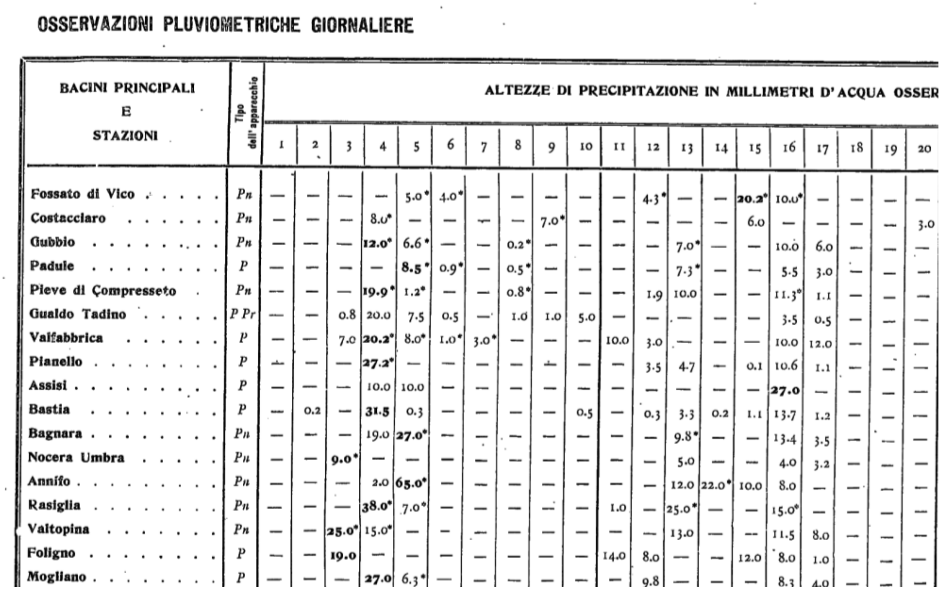
Figure 3. Transcription of manual recording of daily rainfall data during two decades of January 1922 for some rain gauge stations located in central Italy.
3. Rainfall Data Time Resolution at Global Scale
A database with information about the time resolution of rainfall data in different geographic areas of the world was recently published [20]. It provides, for each of the 25,423 rain gauge stations considered from 32 study areas, the complete ta history and the site geographical coordinates (see Figure 4). The main characteristics of the available rainfall observations, grouped by continent, are shown in Table 1.
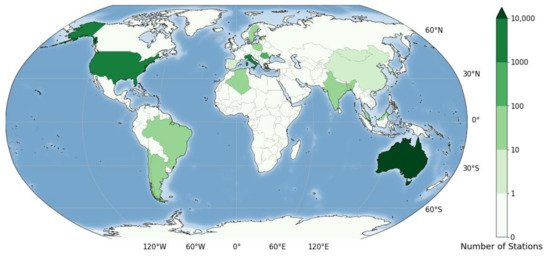
Figure 4. Geographical position of the rain gauge stations considered by Reference [20].
Table 1. Main characteristics of the available rainfall recordings for the rain gauge stations included in the database set up by Reference [20] grouped by continent.
| Continent | Rain Gauges (Number) |
Record Length min/max (Years) |
Beginning of Records (Year) |
Ending of Records (Year) |
Time Resolution min/max (Minutes) |
|---|---|---|---|---|---|
| Africa | 30 | 9/41 | 1968 | 2010 | 1440 |
| America | 5779 | 1/153 | 1867 | 2019 | 1/1440 |
| Asia | 148 | 5/112 | 1879 | 2019 | 1/1440 |
| Australia | 17,768 | 1/180 | 1805 | 2019 | 1/1440 |
| Europe | 1642 | 1/184 | 1805 | 2019 | 1/43,200 |
As is deducible from Table 1, the collected stations are not evenly distributed around the world, but they can be considered a good sample of different monitoring records that can be found in the world (for details see [20]). In a limited number of study areas considered in [20], the length of rainfall data series with known ta is close to 200 years (see Figure 5), while in most areas it is about 100 years. In addition, in a few cases, the ta history is available for recently installed stations.
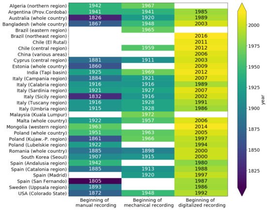
Figure 5. Year of beginning of manual, mechanical, and digital rainfall recordings for the study areas considered in [20].
In many study areas, especially in cases of very old rain gauge stations, recording started by human observation (Figure 5) with coarse time resolution—typically of 1 day but sometimes of 1 month or 1 year. The oldest rainfall data recorded in manual mode (San Fernando station, Spain, since 1805) exhibits ta equal to several days.
Except for a few cases, mechanical recording on paper rolls started in the first decades of the 20th century. For instance, mechanical recordings with ta = 60 min have been carried out at Alghero station (Sardinia region, Italy) since 1927 and at Campulung station (Romania) since 1949.
The introduction of digital data logging took place in the last decades of the 20th century. As a consequence, the investigations of climate change effects on short-duration (sub-hourly) heavy rainfalls are unreliable in almost all geographic areas due to the shortness of rainfall series. Currently, through tipping-bucket sensors, rainfall amounts are recorded in data loggers for each tip time associated with a fixed rainfall depth (0.1 or 0.2 mm). Then, rainfall data can be aggregated with any ta (also equal to 1 min). Borgo S. Lorenzo station (Tuscany region, Italy) and Valletta station (Malta) are two examples of digital data characterized by ta = 1 min recording since 1991 and 2006, respectively. Exceptionally long series of high-resolution rainfall (e.g., Malaysia) were taken out by automatic systems from strip charts of tipping-bucket gauges [1].
Due to the heterogeneity of the database stations, it is hard to synthesize by unique figures and tables the history of all the study areas considered in [20]. In some countries, the history of a single rain gauge is available, as in the case of the Madrid station, while in some others, a network with thousands of rain gauges is involved, as in the case of Australia and Colorado (United States). In any case, Figure 6 attempts to solve the problem by showing the percentage of rain gauges with specific ta for all the stations except those of Australia and Colorado (United States), whose huge numbers would make the plot confusing. From Figure 6, it is possible to deduce that about 50% of stations today have adopted ta = 1 min due to the spread of continuous recording, while data with ta = 1440 min are going to disappear in the near future.
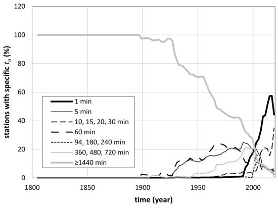
Figure 6. Percentage of rain gauge stations with specific temporal aggregation, ta, as a function of time. All the stations included in the analysis by Reference [20], except those located in Australia and Colorado (United States), are considered.
By the analysis of [20], it is evident that the registration methods of the rain gauge stations changed over time, passing first from daily manual recordings to mechanical recorders with ta equal to 30 min or 1 h, and then to continuous recording with digital data loggers. The changes from one recording type to another were not simultaneous, as both Figure 5 and Figure 6 show.
4. Effect of Rainfall Time Resolution on Estimating Annual Maximum Depths
Errors in the estimates of extreme rainfalls due to different values of d for a specific ta have been widely investigated in the scientific literature. Specifically, it has been shown that for d close to ta, the actual maximum rainfall depth may be underestimated [2][3][4][5][6][7][8][9][10][11][12][13]. Some useful approaches have been published to adjust for this underestimation. For example, Reference [3] observed that for d = ta the results obtained from an analysis based on actual maxima were closely approximated through a frequency analysis of Hd with values multiplied by 1.13. Reference [4], using a probabilistic methodology under the hypothesis of a constant rainfall over the duration of interest, provided a relationship between the sampling ratio, ta/d, and a sampling adjustment factor (SAF). This last quantity is defined as the average ratio of the real maximum rainfall depth for a given d to the maximum one deduced by a fixed recording interval. Reference [10], on the basis of high-temporal-resolution data from 15 rain gauges located in the Kansas City metropolitan area, proposed an empirical relationship between SAF and sampling ratio that provided corrections coherent with other experimental studies (e.g., [21]). However, the limited length of the available rainfall series (in the range 5.3–14.9 years, with average value of 9.6 years) made it impossible to obtain general conclusions. Reference [11] extended the probabilistic methodology used in [4] to temporally variable rainfall distributions and found it to be significantly related to the SAF. A procedure to produce quasi-homogeneous annual maximum rainfall series involving data derived from different time resolutions was recently presented [13]. The authors proposed an algebraic relation that expresses the average underestimation error with the ratio ta/d useful to correct the Hd values. All the aforementioned investigations show that the SAF depends on the sampling ratio as well as on d because the duration influences the shape of the rainfall’s temporal distribution.
4.1. Hyetograph Shape and Hd Underestimation
Following [22][23], indicating by x(t) the rainfall depth observed at time t at a specific site, the cumulative rainfall recorded over a time period d, xd(t), is expressed as:
xd(t)=∫t+dtx(ξ)dξ (1)
and the annual maximum rainfall depth over a duration d is given by:
where t0 is the starting time of each year.
To estimate Hd for each year, the availability of rainfall observations with ta ≤ d is necessary. When d = ta, independently of the rainfall distribution shape, the Hd value can be correctly estimated (Figure 7a) or underestimated (Figure 7b,c) with errors up to 50%.
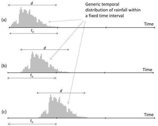
Figure 7. Schematic representation of a generic temporal distribution of rainfall with duration d = ta: (a) condition where a correct evaluation of Hd is possible; (b) condition with a generic underestimate of Hd; (c) condition with the maximum underestimate of Hd (equal to 50%). ta and Hd denote the temporal aggregation and annual maximum rainfall rate of duration d, respectively.
A quantification of the accuracy of a given Hd value is not available, but it is possible to represent the average error for a temporal series with a large number of elements.
For each duration d, this average error depends on both ta and the shape of the rainfall hyetographs. In the case of rectangular shapes, the average underestimate is equal to 25%, because each error value in the range 0–50% has the same probability of occurrence. This result is in accordance with the analysis by [11]. However, as is widely recognized, the Hd values typically belong to heavy rainfalls of erratic shape [24][25][26].
For example, under the hypothesis of a triangular rainfall shape with duration d, the total rainfall depth, Rpd, is:
with h equal to the rainfall intensity peak.
In case of ta = d, the underestimation error of a single Hd is still in the range 0–50%, but the associated average value, Ea, derived by integrating through the rainfall duration (see also [11]) becomes:
This quantity, expressed in terms of rainfall depth percentage, is expressed as:
such that for ta = d is equal to 16.67%, in accordance with the results in [11].
Experimental evidence from different rain gauge stations and d values indicate a steeper trend of rainfall before and after the peak; thus, the actual values of Ea% should assume values lower than 16.67%.
In any case, independently of the adopted ta, underestimation errors in determining the Hd values cannot be eliminated. The average error Ea% decreases if the ratio ta/d decreases. Specifically, from Equations (3) and (5), it can be expressed as:
becoming negligible for sufficiently small ta/d.
On this basis, for d = ta = 1 min, in the case of an extreme rainfall with rate of 300 mm/h, the underestimation error is lower than 1 mm. In addition, as the durations of interest for Hd are generally ≥5 min, rainfall observations with ta = 1 min may be considered to have negligible error.
4.2. Correction Procedure for Hd Series
When rainfall records are characterized by coarse time resolution, the underestimation error in the determination of the annual maximum rainfall depth for a fixed d can be considered as a random variable following an exponential probability distribution with entity inversely correlated to Hd [27]. Correction through the use of the average error has relevant effects only if it involves a large number of underestimated values. For example, Reference [13] proposed a lower limit of 15–20 years for the series length to obtain a reliable estimate of the average error, especially when d ≈ ta, because for shorter series the error exhibits an irregular trend. The last outcome is in contrast with the analysis by Young and McEnroe [10], who considered rainfall depth series of about 10 years in length.
An overall analysis of the available studies suggests that:
-
On a specific value, the underestimation error has a random behaviour and is within 50%;
-
The average error depends on both ta/d and d;
-
The average error can be approximately supposed independent from the device location;
-
The largest value of the average error occurs for d = ta and is theoretically less than or equal to 16.67%;
In the case of d = nta, the average error is less than or equal to (1/n) × 16.67%.
The aforementioned error considers the effect of time resolution on Hd values, either for a single year or for historical series. The described procedure allows for an increase in the homogeneity of Hd data series deriving from rainfall observations characterized by very different temporal aggregations.
Figure 8 shows the relationships proposed in[4][10][13] to quantify the average underestimation with variable ratio ta/d. Reference[4] originally proposed the function expressed as:
Ea%=12.501tad (%)
and considered a probabilistic approach assuming a constant rainfall rate through the duration, while Young and McEnroe[10] , by using Hd observed series, derived the following relation:
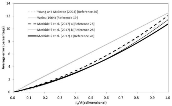
Figure 8. Average underestimation error of the annual maximum rainfall depth for different values of the ratio between time resolution, ta, and duration, d, obtained by Equation (7) [4], Equation (8) [10], and Equations (9)–(11) [13]. In this last case, symbols “a”, “b”, and “c” stand for d ≤ 30 min, d in the interval between 30 and 180 min, and d ≥ 180 min, respectively.
Lastly, on the basis of the relationship between d and the rainfall shape that affects the error entity [11], Reference [13] proposed the following relations:
Relations (9–11) make it possible to correct the Hd series derived from data with coarse ta as a function of d and ta/d.
In principle, the relations by Reference [13] should be more effective because they make it possible to also consider the shape of the temporal distribution of rainfall in determining the correction factor. Along this line, Figure 8 shows that the equation from Reference [4] mainly produces larger average errors for intermediate values of the ratio ta/d. On the contrary, the equation of Young and McEnroe [10], although also calibrated with very short data series, provides results comparable to those of Reference [13].
5. Role of ta in Hydrological Applications
The observed heterogeneity in the ta characteristic as a function of the considered geographic zone and epoch can affect further analyses based on Hd values, such as the determination of intensity–duration–frequency curves.
Specifically, the usage of long Hd series with underestimated elements for the determination of rainfall depth–duration–frequency curves produces errors of variable magnitude (up to 10%) with different return periods and rainfall duration [13]. These errors become relevant when the Hd series contain elements derived from a temporal aggregation much greater than 1 min. In addition, when designing hydraulic structures or restructuring existing ones, the effects on heavy rainfalls produced by climate change have to be considered, taking into account possible distortions due to the above errors in the Hd series.
In this context, [14] highlighted that the coarse time resolution of rainfall observations can substantially influence the results of widely used statistical techniques applied to check the possible effects of climate change on extreme rainfalls, such as, e.g., the least-square linear approach, the Mann–Kendall test, the Spearman test, and Sen’s method. The following major insights were derived:
-
Underestimation errors caused by coarse time resolution produce significant effects on least-squares linear trend analysis. The usage of a correction factor for the Hd values, independent of the selected approach, can make the trend sign change from positive to negative, and the effects are more evident for series with larger numbers of elements with ta/d = 1.
-
The non-parametric Mann–Kendall test[28][29] and the Spearman rank correlation test[30] , with significance level equal to 0.05, exhibit a negligible sensitivity to underestimation errors on the Hd values.
-
The application of Sen’s method[31] gives different outcomes depending on whether uncorrected or corrected Hd values are considered
-
Because analysis of possible climatic trends requires data series at least 60 years long to include the effect of large-scale climate oscillations (see also[32] ), it is not feasible to consider only rainfall data with ta = 1 min that have historical series of only two/three decades in most geographic zones (see also[20]).
-
Common homogeneity tests such as the standard normal homogeneity test for a single break point[33] or the Pettitt test[34] are not capable of detecting discontinuities in Hd series determined by different time resolutions. This result can be justified with the hypothesis that for annual maximum rainfall data, underestimation errors do not produce sufficiently relevant break points.
References
- Deidda, R.; Mascaro, G.; Piga, E.; Querzoli, G. An automatic system for rainfall signal recognition from tipping bucket gage strip charts. J. Hydrol. 2007, 333, 400–412.
- Hershfield, D.M.; Wilson, W.T. Generalizing of Rainfall-Intensity-Frequency Data. In IUGG/IAHS Publication No. 43; 1958; pp. 499–506. Available online: (accessed on 2 November 2020).
- Hershfield, D.M. Rainfall frequency atlas of the United States for durations from 30 minutes to 24 hours and return periods from 1 to 100 years. In US Weather Bureau Technical Paper N. 40; U.S. Department of Commerce: Washington, DC, USA, 1961.
- Weiss, L.L. Ratio of true to fixed-interval maximum rainfall. J. Hydraul. Div. 1964, 90, 77–82.
- Harihara, P.S.; Tripathi, N. Relationship of the clock-hour to 60-min and the observational day to 1440-min rainfall. Ind. J. Meteorol. Geophys. 1973, 24, 279–282.
- Natural Environment Research Council. Flood Studies Report; Natural Environment Research Council: London, UK, 1975.
- Van Montfort, M.A.J. Sliding maxima. J. Hydrol. 1990, 118, 77–85.
- Faiers, G.E.; Grymes, J.M.; Keim, B.D.; Muller, R.A. A re-examination of extreme 24 hour rainfall in Louisiana, USA. Clim. Res. 1994, 4, 25–31.
- Van Montfort, M.A.J. Concomitants of the Hershfield factor. J. Hydrol. 1997, 194, 357–365.
- Young, C.B.; McEnroe, B.M. Sampling adjustment factors for rainfall recorded at fixed time intervals. J. Hydrol. Eng. 2003, 8, 294–296.
- Yoo, C.; Park, M.; Kim, H.J.; Choi, J.; Sin, J.; Jun, C. Classification and evaluation of the documentary-recorded storm events in the Annals of the Choson Dynasty (1392–1910), Korea. J. Hydrol. 2015, 520, 387–396.
- Papalexiou, S.M.; Dialynas, Y.G.; Grimaldi, S. Hershfield factor revisited: Correcting annual maximum precipitation. J. Hydrol. 2016, 524, 884–895.
- Morbidelli, R.; Saltalippi, C.; Flammini, A.; Cifrodelli, M.; Picciafuoco, T.; Corradini, C.; Casas-Castillo, M.C.; Fowler, H.J.; Wilkinson, S.M. Effect of temporal aggregation on the estimate of annual maximum rainfall depths for the design of hydraulic infrastructure systems. J. Hydrol. 2017, 554, 710–720.
- Morbidelli, R.; Saltalippi, C.; Flammini, A.; Corradini, C.; Wilkinson, S.M.; Fowler, H.J. Influence of temporal data aggregation on trend estimation for intense rainfall. Adv. Water Resour. 2018, 122, 304–316.
- Sevruk, B.; Klemm, S. Catalogue of national standard precipitation gauges. Instruments and observing methods. In Report No. 39, WMO/TD-No. 313; 1989; Available online: (accessed on 2 November 2020).
- New, M.; Todd, M.; Hulme, M.; Jones, P.D. Precipitation measurements and trends in the twentieth century. Int. J. Climatol. 2001, 21, 1899–1922.
- Strangeways, I. Precipitation: Theory, Measurement and Distribution; Cambridge University Press: Cambridge, UK, 2007; ISBN 13978-0-521-85117-6.
- Kidd, C.; Becker, A.; Huffman, G.J.; Muller, C.L.; Joe, P.; Skofronick-Jackson, G.; Kirschbaum, D.B. So, how much of the Earth’s surface is covered by rain gauges? Bull. Am. Meteorol. Soc. 2017, 98, 69–78.
- Sun, Q.; Miao, C.; Duan, Q.; Ashouri, H.; Sorooshian, S.; Hsu, K.-L. A review of global precipitation data sets: Data sources, estimation, and intercomparisons. Rev. Geophys. 2018, 56, 79–107.
- Morbidelli, R.; García-Marín, A.P.; Al Mamun, A.; Atiqur, R.M.; Ayuso-Muñoz, J.L.; Bachir Taouti, M.; Baranowski, P.; Bellocchi, G.; Sangüesa-Pool, C.; Bennett, B.; et al. The history of rainfall data time-resolution in different geographical areas of the world. J. Hydrol. 2020, 590, 125258.
- Miller, J.F.; Frederick, R.H.; Tracey, R.J. Precipitation-Frequency Atlas of the Western United States; NOAA Atlas 2; National Weather Service, National Oceanic and Atmospheric Administration, U.S. department of Commerce: Washington, DC, USA, 1973.
- Burlando, P.; Rosso, R. Scaling and multiscaling models of depth-duration-frequency curves for storm precipitation. J. Hydrol. 1996, 187, 45–64.
- Boni, G.; Parodi, A.; Rudari, R. Extreme rainfall events: Learning from raingauge time series. J. Hydrol. 2006, 327, 304–314.
- Balme, M.; Vischel, T.; Lebel, T.; Peugeot, C.; Galle, S. Assessing the water balance in the Sahel: Impact of small scale rainfall variability on runoff, Part 1: Rainfall variability analysis. J. Hydrol. 2006, 331, 336–348.
- Al-Rawas, G.A.; Valeo, C. Characteristics of rainstorm temporal distributions in arid mountainous and coastal regions. J. Hydrol. 2009, 376, 318–326.
- Coutinho, J.V.; Almeida, C.D.N.; Leal, A.M.F.; Barbosa, L.R. Characterization of sub-daily rainfall properties in three rainfall gauges located in Northeast of Brazil. Evolving Water Resources Systems: Understanding, Predicting and Managing Water-Society Interactions. Proc. Int. Assoc. Hydrol. Sci. 2014, 364, 345–350.
- Morbidelli, R.; Saltalippi, C.; Flammini, A.; Picciafuoco, T.; Dari, J.; Corradini, C. Characteristics of the underestimation error of annual maximum rainfall depth due to coarse temporal aggregation. Atmosphere 2018, 9, 303.
- Mann, H.B. Nonparametric tests against trend. Econometrica 1945, 13, 46–59.
- Kendall, M.G. Rank Correlation Methods; Griffin: London, UK, 1975.
- Khaliq, M.N.; Ouarda, T.B.M.J.; Gachon, P.; Sushama, L.; St-Hilaire, A. Identification of hydrological trends in the presence of serial and cross correlation: A review of selected methods and their application to annual flow regimes of Canadian rivers. J. Hydrol. 2009, 368, 117–130.
- Sen, Z. Innovative trend analysis methodology. J. Hydrol. Eng. 2012, 17, 1042–1046.
- Willems, P. Adjustment of extreme rainfall statistics accounting for multidecadal climate oscillations. J. Hydrol. 2013, 490, 126–133.
- Alexandersson, H. A homogeneity test applied to precipitation data. J. Climatol. 1986, 6, 661–675.
- Pettitt, A.N. A non-parametric approach to the change-point detection. Appl. Stat. 1979, 28, 126–135.

