As is widely recognized, rainfall data is necessary for the mathematical modelling of extreme hydrological events, such as droughts or floods, as well as for evaluating surface and subsurface water resources and their quality. The phase, quantity, and elevation of generic hydrometeors in the atmosphere can be estimated by ground-based radars. Satellites can provide images with visible and infrared radiation, and they can also serve as platforms for radiometers to derive the quantity and phase of hydrometeors. Radars and satellites provide spatial information on precipitation at wide scales, avoiding many problems connected to local ground measurements, including those for the areal inhomogeneity of a network. However, direct rainfall observations at point scale can be obtained only by rain gauges installed at the soil surface.
- rainfall data measurements
- rainfall time resolution
- rainfall data
1. Recording of rainfall data
[1]
ta
ta
Hd
d
[2][3][4][5][6][7][8][9][10][11][12][13]
d
ta,
Hd
Hd
ta
[13]
[14]
[2][3][4][5][6][7][8][9][10][11][12][13]
Hd
d
[14]
ta
Hd
2. Rainfall Data Characteristics
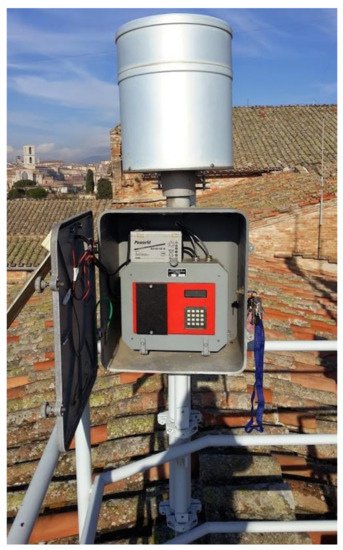
Figure 1.
ta
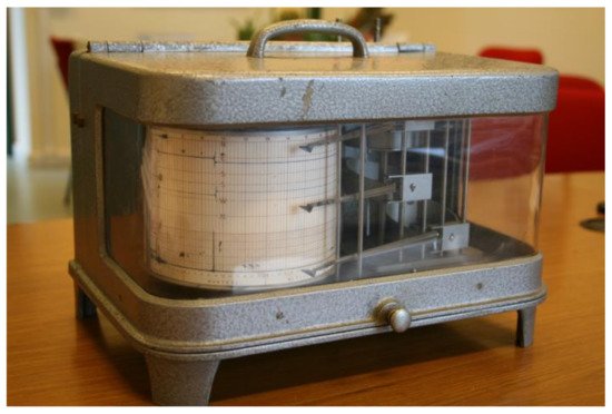
Figure 2.
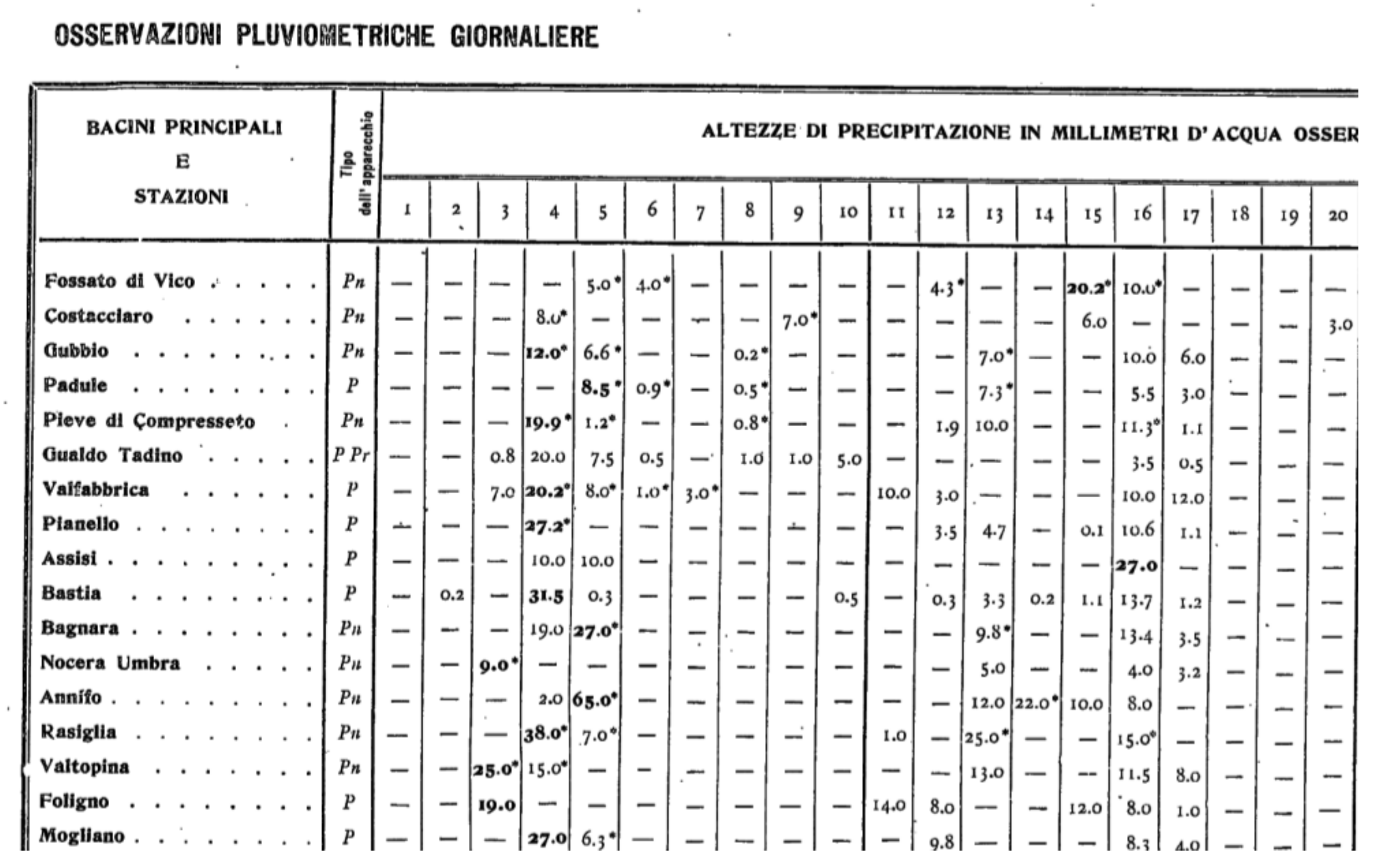
Figure 3.
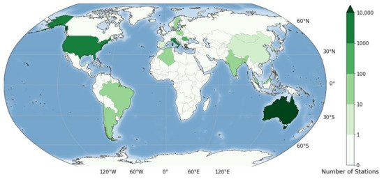
3. Rainfall Data Time Resolution at Global Scale
[20]
ta
Table 1.
[20]
| Continent | Rain Gauges (Number) |
Record Length min/max (Years) |
Beginning of Records (Year) |
Ending of Records (Year) |
Time Resolution min/max (Minutes) |
|---|
| Africa | 30 | 9/41 | 1968 | 2010 | 1440 |
| America | 5779 | 1/153 | 1867 | 2019 | 1/1440 |
| Asia | 148 | 5/112 | 1879 | 2019 | 1/1440 |
| Australia |
where
t0 is the starting time of each year.
To estimate
Hd
ta
d
d
ta
Hd
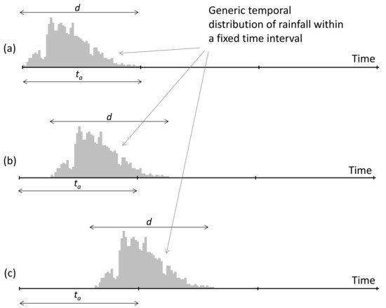
Figure 7.
d
ta
a
Hd
b
Hd
c
Hd
ta
Hd
d
Hd
d
ta
[11]
Hd
d
Rpd
with
h equal to the rainfall intensity peak.
In case of
ta
d
Hd
Ea
[11]
This quantity, expressed in terms of rainfall depth percentage, is expressed as:
such that for
ta
d
[11]
d
Ea%
ta
Hd
Ea%
ta
d
ta
d
d
ta
Hd
ta = 1 min may be considered to have negligible error.
4.2. Correction Procedure for Hd Series
d
Hd
[27]
[13]
d
ta
[10]
-
On a specific value, the underestimation error has a random behaviour and is within 50%;
-
The average error depends on both ta/d and d;
| 17,768 |
| 1/180 |
| 1805 |
| 2019 |
| 1/1440 |
| Europe | |||
| 1642 | |||
| 1/184 | 1805 | 2019 | 1/43,200 |
[20]
[20]
ta
ta
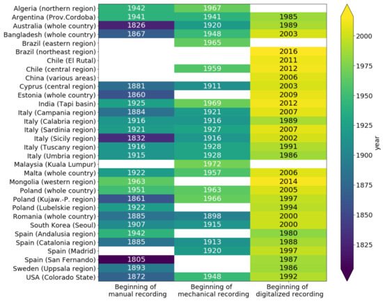
Figure 5.
[20]
ta
ta
ta
ta
[1]
[20]
ta
ta
ta
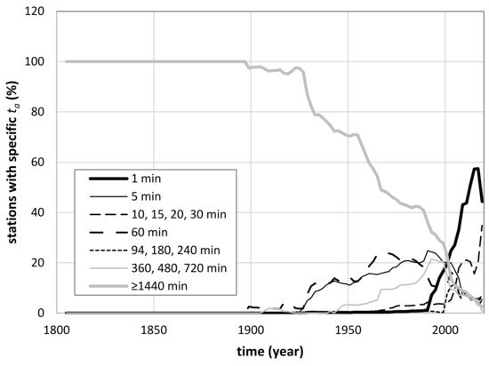
Figure 6.
ta
[20]
[20]
ta
4. Effect of Rainfall Time Resolution on Estimating Annual Maximum Depths
d
ta
d
ta
[2][3][4][5][6][7][8][9][10][11][12][13]
[3]
d
ta
Hd
[4]
ta
d
d
[10]
[21]
[11]
[4]
[13]
ta
d
Hd
d
4.1. Hyetograph Shape and Hd Underestimation
x
t
t
d
xd
t
xd(t)=∫t+dtx(ξ)dξ (1)
and the annual maximum rainfall depth over a duration
d
-
The average error can be approximately supposed independent from the device location;
-
The largest value of the average error occurs for d = ta and is theoretically less than or equal to 16.67%;
In the case of
- -
-
On a specific value, the underestimation error has a random behaviour and is within 50%;
- -
-
The average error depends on both ta/d and d;
- -
-
The average error can be approximately supposed independent from the device location;
- -
-
The largest value of the average error occurs for d = ta and is theoretically less than or equal to 16.67%;
- -
-
In the case of
d
=nta
, the average error is less than or equal to (1/n) × 16.67%.
) × 16.67%.
Hd
Hd
Figure 8 shows the relationships proposed in
shows the relationships proposed in[4][10][13] to quantify the average underestimation with variable ratio
to quantify the average underestimation with variable ratiota
/d. Reference
. Reference[4]
originally proposed the function expressed as:Ea%
tad (%)
and considered a probabilistic approach assuming a constant rainfall rate through the duration, while Young and McEnroe
and considered a probabilistic approach assuming a constant rainfall rate through the duration, while Young and McEnroe[10] , by using
, by usingHd observed series, derived the following relation:
observed series, derived the following relation: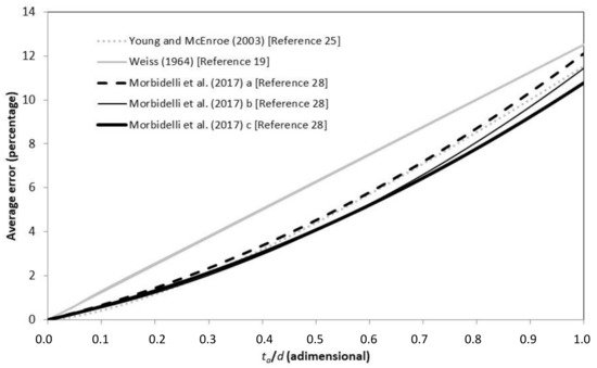
Figure 8.
ta
d
[4]
[10]
[13]
d
d
d
d
[11]
[13]
Hd
ta
d
ta
d
[13]
[4]
ta
d
[10]
[13]
5. Role of ta in Hydrological Applications
ta
Hd
Hd
[13]
Hd
Hd
[14]
-
Underestimation errors caused by coarse time resolution produce significant effects on least-squares linear trend analysis. The usage of a correction factor for the Hd values, independent of the selected approach, can make the trend sign change from positive to negative, and the effects are more evident for series with larger numbers of elements with ta/d = 1.
-
The non-parametric Mann–Kendall test[28][29] and the Spearman rank correlation test[30] , with significance level equal to 0.05, exhibit a negligible sensitivity to underestimation errors on the Hd values.
-
The application of Sen’s method[31] gives different outcomes depending on whether uncorrected or corrected Hd values are considered
-
Because analysis of possible climatic trends requires data series at least 60 years long to include the effect of large-scale climate oscillations (see also[32] ), it is not feasible to consider only rainfall data with ta = 1 min that have historical series of only two/three decades in most geographic zones (see also[20]).
-
Common homogeneity tests such as the standard normal homogeneity test for a single break point[33] or the Pettitt test[34] are not capable of detecting discontinuities in Hd series determined by different time resolutions. This result can be justified with the hypothesis that for annual maximum rainfall data, underestimation errors do not produce sufficiently relevant break points.
- -
-
Underestimation errors caused by coarse time resolution produce significant effects on least-squares linear trend analysis. The usage of a correction factor for the Hd values, independent of the selected approach, can make the trend sign change from positive to negative, and the effects are more evident for series with larger numbers of elements with ta/d = 1.
- -
-
The non-parametric Mann–Kendall test [28][29] and the Spearman rank correlation test [30], with significance level equal to 0.05, exhibit a negligible sensitivity to underestimation errors on the Hd values.
- -
-
The application of Sen’s method [31] gives different outcomes depending on whether uncorrected or corrected Hd values are considered.
- -
-
Because analysis of possible climatic trends requires data series at least 60 years long to include the effect of large-scale climate oscillations (see also [32]), it is not feasible to consider only rainfall data with ta = 1 min that have historical series of only two/three decades in most geographic zones (see also [20]).
- -
-
Common homogeneity tests such as the standard normal homogeneity test for a single break point [33] or the Pettitt test [34] are not capable of detecting discontinuities in Hd series determined by different time resolutions. This result can be justified with the hypothesis that for annual maximum rainfall data, underestimation errors do not produce sufficiently relevant break points.
References
- Deidda, R.; Mascaro, G.; Piga, E.; Querzoli, G. An automatic system for rainfall signal recognition from tipping bucket gage strip charts. J. Hydrol. 2007, 333, 400–412.
- Hershfield, D.M.; Wilson, W.T. Generalizing of Rainfall-Intensity-Frequency Data. In IUGG/IAHS Publication No. 43; 1958; pp. 499–506. Available online: (accessed on 2 November 2020).
- Hershfield, D.M. Rainfall frequency atlas of the United States for durations from 30 minutes to 24 hours and return periods from 1 to 100 years. In US Weather Bureau Technical Paper N. 40; U.S. Department of Commerce: Washington, DC, USA, 1961.
- Weiss, L.L. Ratio of true to fixed-interval maximum rainfall. J. Hydraul. Div. 1964, 90, 77–82.
- Harihara, P.S.; Tripathi, N. Relationship of the clock-hour to 60-min and the observational day to 1440-min rainfall. Ind. J. Meteorol. Geophys. 1973, 24, 279–282.
- Natural Environment Research Council. Flood Studies Report; Natural Environment Research Council: London, UK, 1975.
- Van Montfort, M.A.J. Sliding maxima. J. Hydrol. 1990, 118, 77–85.
- Faiers, G.E.; Grymes, J.M.; Keim, B.D.; Muller, R.A. A re-examination of extreme 24 hour rainfall in Louisiana, USA. Clim. Res. 1994, 4, 25–31.
- Van Montfort, M.A.J. Concomitants of the Hershfield factor. J. Hydrol. 1997, 194, 357–365.
- Young, C.B.; McEnroe, B.M. Sampling adjustment factors for rainfall recorded at fixed time intervals. J. Hydrol. Eng. 2003, 8, 294–296.
- Yoo, C.; Park, M.; Kim, H.J.; Choi, J.; Sin, J.; Jun, C. Classification and evaluation of the documentary-recorded storm events in the Annals of the Choson Dynasty (1392–1910), Korea. J. Hydrol. 2015, 520, 387–396.
- Papalexiou, S.M.; Dialynas, Y.G.; Grimaldi, S. Hershfield factor revisited: Correcting annual maximum precipitation. J. Hydrol. 2016, 524, 884–895.
- Morbidelli, R.; Saltalippi, C.; Flammini, A.; Cifrodelli, M.; Picciafuoco, T.; Corradini, C.; Casas-Castillo, M.C.; Fowler, H.J.; Wilkinson, S.M. Effect of temporal aggregation on the estimate of annual maximum rainfall depths for the design of hydraulic infrastructure systems. J. Hydrol. 2017, 554, 710–720.
- Morbidelli, R.; Saltalippi, C.; Flammini, A.; Corradini, C.; Wilkinson, S.M.; Fowler, H.J. Influence of temporal data aggregation on trend estimation for intense rainfall. Adv. Water Resour. 2018, 122, 304–316.
- Sevruk, B.; Klemm, S. Catalogue of national standard precipitation gauges. Instruments and observing methods. In Report No. 39, WMO/TD-No. 313; 1989; Available online: (accessed on 2 November 2020).
- New, M.; Todd, M.; Hulme, M.; Jones, P.D. Precipitation measurements and trends in the twentieth century. Int. J. Climatol. 2001, 21, 1899–1922.
- Strangeways, I. Precipitation: Theory, Measurement and Distribution; Cambridge University Press: Cambridge, UK, 2007; ISBN 13978-0-521-85117-6.
- Kidd, C.; Becker, A.; Huffman, G.J.; Muller, C.L.; Joe, P.; Skofronick-Jackson, G.; Kirschbaum, D.B. So, how much of the Earth’s surface is covered by rain gauges? Bull. Am. Meteorol. Soc. 2017, 98, 69–78.
- Sun, Q.; Miao, C.; Duan, Q.; Ashouri, H.; Sorooshian, S.; Hsu, K.-L. A review of global precipitation data sets: Data sources, estimation, and intercomparisons. Rev. Geophys. 2018, 56, 79–107.
- Morbidelli, R.; García-Marín, A.P.; Al Mamun, A.; Atiqur, R.M.; Ayuso-Muñoz, J.L.; Bachir Taouti, M.; Baranowski, P.; Bellocchi, G.; Sangüesa-Pool, C.; Bennett, B.; et al. The history of rainfall data time-resolution in different geographical areas of the world. J. Hydrol. 2020, 590, 125258.
- Miller, J.F.; Frederick, R.H.; Tracey, R.J. Precipitation-Frequency Atlas of the Western United States; NOAA Atlas 2; National Weather Service, National Oceanic and Atmospheric Administration, U.S. department of Commerce: Washington, DC, USA, 1973.
- Burlando, P.; Rosso, R. Scaling and multiscaling models of depth-duration-frequency curves for storm precipitation. J. Hydrol. 1996, 187, 45–64.
- Boni, G.; Parodi, A.; Rudari, R. Extreme rainfall events: Learning from raingauge time series. J. Hydrol. 2006, 327, 304–314.
- Balme, M.; Vischel, T.; Lebel, T.; Peugeot, C.; Galle, S. Assessing the water balance in the Sahel: Impact of small scale rainfall variability on runoff, Part 1: Rainfall variability analysis. J. Hydrol. 2006, 331, 336–348.
- Al-Rawas, G.A.; Valeo, C. Characteristics of rainstorm temporal distributions in arid mountainous and coastal regions. J. Hydrol. 2009, 376, 318–326.
- Coutinho, J.V.; Almeida, C.D.N.; Leal, A.M.F.; Barbosa, L.R. Characterization of sub-daily rainfall properties in three rainfall gauges located in Northeast of Brazil. Evolving Water Resources Systems: Understanding, Predicting and Managing Water-Society Interactions. Proc. Int. Assoc. Hydrol. Sci. 2014, 364, 345–350.
- Morbidelli, R.; Saltalippi, C.; Flammini, A.; Picciafuoco, T.; Dari, J.; Corradini, C. Characteristics of the underestimation error of annual maximum rainfall depth due to coarse temporal aggregation. Atmosphere 2018, 9, 303.
- Mann, H.B. Nonparametric tests against trend. Econometrica 1945, 13, 46–59.
- Kendall, M.G. Rank Correlation Methods; Griffin: London, UK, 1975.
- Khaliq, M.N.; Ouarda, T.B.M.J.; Gachon, P.; Sushama, L.; St-Hilaire, A. Identification of hydrological trends in the presence of serial and cross correlation: A review of selected methods and their application to annual flow regimes of Canadian rivers. J. Hydrol. 2009, 368, 117–130.
- Sen, Z. Innovative trend analysis methodology. J. Hydrol. Eng. 2012, 17, 1042–1046.
- Willems, P. Adjustment of extreme rainfall statistics accounting for multidecadal climate oscillations. J. Hydrol. 2013, 490, 126–133.
- Alexandersson, H. A homogeneity test applied to precipitation data. J. Climatol. 1986, 6, 661–675.
- Pettitt, A.N. A non-parametric approach to the change-point detection. Appl. Stat. 1979, 28, 126–135.

