 +1 credit
| Version | Summary | Created by | Modification | Content Size | Created at | Operation |
|---|---|---|---|---|---|---|
| 1 | Lorentz Jäntschi | + 1553 word(s) | 1553 | 2019-07-10 09:40:49 | | | |
| 2 | Lorentz Jäntschi | + 1573 word(s) | 1573 | 2019-07-10 11:13:36 | | | | |
| 3 | Lorentz Jäntschi | + 1573 word(s) | 1573 | 2019-07-10 11:18:21 | | | | |
| 4 | Lorentz Jäntschi | + 1577 word(s) | 1577 | 2019-07-10 11:23:56 | | | | |
| 5 | Lorentz Jäntschi | + 1577 word(s) | 1577 | 2019-07-10 11:28:40 | | | | |
| 6 | Lorentz Jäntschi | + 6 word(s) | 1583 | 2019-07-10 11:31:49 | | | | |
| 7 | Lorentz Jäntschi | + 27 word(s) | 1604 | 2019-07-11 05:35:47 | | | | |
| 8 | Bruce Ren | -47 word(s) | 1557 | 2020-10-29 05:19:58 | | |
Video Upload Options
One of the pillars of experimental sciences is sampling. Based on analysis conducted on samples the estimations for the populations are made. The distributions are split in two main groups: continuous and discrete and the present study applies for the continuous ones. One of the challenges of the sampling is the accuracy of it, or, in other words how representative is the sample for the population from which was drawn. Another challenge, connected with this one, is the presence of the outliers - observations wrongly collected, not actually belonging to the population subjected to study. The present study proposes a statistic (and a test) intended to be used for any continuous distribution to detect the outliers, by constructing the confidence interval for the extreme value in the sample, at certain (preselected) risk of being in error, and depending on the sample size. The proposed statistic is operational for known distributions (having known their probability density function) and is dependent too on the statistical parameters of the population.
1. Introduction
Many statistical techniques are sensitive to the presence of outliers and all calculations, including the mean and standard deviation may be distorted by a single grossly inaccurate data point and therefore checking for outliers should be a routine part of any data analysis.
Several tests were developed to date for the purpose of identifying outliers of certain distributions. Most of the studies are connected with the Normal (or Gauss) distribution (Gauss, 1809)[1]. Probably the first paper which attracted attention on this matter is (Tippett, 1925)[2] followed by the derivation of the distribution of the extreme values in samples taken from Normal distribution (Fisher & Tippett, 1928)[3]. Later, a series of tests were developed - probably the first being (Thompson, 1935)[4], subjected to evaluation (Pearson & Sekar, 1936)[5], and revised (Grubbs, 1950)[6], (Grubbs, 1969)[7].
For other distributions such as Gamma distribution procedures for detecting outliers were proposed (Nooghabi, et al., 2010)[8], revised (Kumar & Lalitha, 2012)[9], and unfortunately proved not efficient (Lucini & Frery, 2017)[10].
The first attempt to generalize the criterion for detecting the outliers for any distribution is (Hartley, 1942)[11], but unfortunately the researches on this subject are very scarce and a notable recent attempt should be noted (Bardet & Dimby, 2017)[12].
In (Jäntschi 2019)[13] is proposed a method for constructing the confidence intervals for the extreme values of any continuous distribution for which also the cumulative distribution function is obtainable. The method have as direct application a simple test for detecting the outliers. The proposed method is based on deriving the statistic for the extreme values for the uniform distribution.
When a sample of data is tested under the null hypothesis that it follows a certain distribution, it is intrinsically assumed that the distribution is known. The usual assumption is that we possess its probability density function (PDF; for a continuous distribution).
When the PDF is (possibly intrinsically) known, it is not necessary that its (statistical) parameters are known, and here a complex problem of estimating the parameters of the (population) distribution from the sample can be (re)opened.
The estimation of the parameters of the distribution of the data is, in general, biased by the presence of the outliers in the data, and thus, identifying the outliers along with the estimation of the parameters of the distribution is a difficult task operating on two statistical hypotheses.
Taking the general case, for (x1, …, xn) as n independent draws (or observations) from a (assumed known) continuous distribution defined by its probability density function, PDF(x; (πj)1≤£j≤m) where (πj)1≤j≤m are the (assumed unknown) m statistical parameters of the distribution, by the way of integration for a (assumed known) domain ("D") of the distribution we may have access to the associated cumulative density function ("CDF") CDF(x; (πj)1≤j≤m; "PDF"), expressed as (eq.1):
\( CDF(x; (\pi_j)_{1 \leq j \leq m}; \text{"PDF")} = \int_{inf(D)}^{x}{PDF(t; (\pi_j)_{1 \leq j \leq m})dt} \)
where inf(D) were used in the disfavor of min(D) to include unbounded domains (e.g. when inf(D) = -∞). Please note that having the PDF and CDF does not necessary implies that we have an explicit formula (or expression) for any of them. But with access to numerical integration methods (Davis & Rabinowitz, 1975)[14] it's enough to have the possibility to evaluate them in any point (x).
Unlike PDF(x), CDF(x) is a bijective function and therefore is invertible all the time (even if we don't have explicit formula; let "InvCDF" being its inverse, eq.2):
\( \text{if } CDF(x; (\pi_j)_{1 \leq j \leq m}; \text{"PDF")} \text{ then } x = InvCDF(p; (\pi_j)_{1 \leq j \leq m}; \text{"PDF")} \text{ and vice-versa} \)
CDF(x; (πj)1≤j≤m; "PDF") is a strong tool simplifying a lot the problem at hand: the problem of analyzing any distribution function (PDF) is translated into analyzing only one (the continuous uniform distribution) when the series of observed data (xi)1≤i≤n is expressed through their associated probabilities pi = CDF(xi) (for 1≤i≤n) and the analysis can be conducted on the (pi)1≤i≤n series instead (eq.3).
\( p_i \leftarrow CDF(x_i; (\pi_j)_{1 \leq j \leq m}; \text{"PDF"}) \text{ for } 1 \leq i \leq n\)
2. Extreme values sample statistic
A statistic called g1 was developed to be applicable to any distribution. For a series of probabilities ((pi)1≤i≤n) the (ri)1≤i≤n differences are calculated (eq.4):
\( r_i \leftarrow |p_i-0.5| \text{ for } 1 \leq i \leq n \)
The g1 statistic is then calculated as (eq.5):
\( g1 \leftarrow \max\limits_{1 \leq i \leq n}r_i \)
3. Extreme values population statistic
The g1 statistic have a very simple calculation formula (see eq. 5) and, as expected, also its CDF formula is very simple (see eq.6). Thus, for a calculated sample statistic g1 (x ← g1 in eq.5), the significance level (α ← 1-p) is immediate (eq.6).
\( p = CDF_{g1}(x; n) = P(X \leq x \text{ | X follows g1}) = (2\cdot x)^n, \, \alpha = 1-p = 1- (2\cdot x)^n \)
On the regard of the g1 statistic, the domain for a variable distributed by g1 statistic (see eq.6) have the values between 0 and 0.5 with the mode at p = 0 (a vertical asymptote at p = 0), a median of n-1·2-1/n (and having a left asymmetry decreasing with the increasing of n and converging - for n → ∞ - to symmetry) and mean of 1/2(n+1).
The expression of CDFg1 is easy to be inverted (eq.7).
\( CDF_{g1}(x; n) = (2x)^n \rightarrow InvCDF_{g1}(p; n) = \sqrt[n]{p}/2 \)
Eq.7 can be used to calculate critical values of the g1 statistic for any values of α (α ← 1-p) and n. The critical values of g1 statistic acts as the boundaries of the confidence intervals.
4. Monte-Carlo simulation
For convenience, in the figure (from [13]) is represented the value of the estimation error in each observation point (999 points corresponding to p = 0.001 to p = 0.999 for each n from 2 to 12) from a MC simulation intended to proof the connection between (5) and (6).
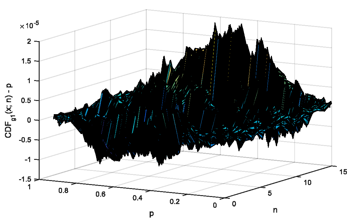 Figure. Departures between expected and observed probabilities for g1 statistic (eq.5 vs. eq.6)
5. Extreme values confidence interval
By setting the risk of being in error α (usually at 5%) then p = 1-α and eq.7 can be used to calculate the statistic associated with it (InvCDFg1(1-α; n)). By replacing this value into eqs. (5) & (6) the (extreme) probabilities can be extracted (eq.8).
\( \max\limits_{1 \leq i \leq n}|p_i-0.5| = \sqrt[n]{1-\alpha}/2 \rightarrow p_{extreme}(\alpha) = 0.5 \pm \sqrt[n]{1-\alpha}/2 \)
In order to arrive at the confidence intervals for the extreme values in the sampled data (eq.9) is necessary to use (again) the inverse of the CDF, and at this time for the distribution of the sampled data.
\( x_{extreme}(\alpha) = InvCDF(0.5 \pm \sqrt[n]{1-\alpha}/2; (\pi_j)_{1 \leq j \leq m}); \text{"PDF"}) \)
6. Testing samples for outliers
To illustrate the arriving at the confidence intervals for the extreme values in the sampled data, and the use of the statistic as a test detecting the outliers, two examples are given. First is based on Table 4 from [13], and the second on Table 11 from [13].
The same data were tested against the assumption that follows a generalized Gauss-Laplace distribution (eq.10) and a normal (Gauss) distribution (eq.11).
\( PDF_{GL}(x; \mu,\sigma,\kappa) = c_1\sigma^{-1}e^{-|c_0z|^\kappa}, \, c_0 = \Big( \frac{\Gamma(3/\kappa)}{\Gamma(1/\kappa)}\Big)^{1/2}, \, c_1 = \frac{\kappa c_0}{2\Gamma(1/\kappa)}, \, z = \frac{x-\mu}{\sigma} \)
\( PDF_G(x; \mu,\sigma) = \sigma^{-1}(2\pi)^{-1/2}e^{-\frac{(x-\mu)^2}{\sigma^2}} \)
The (sorted) sample of data is: {4.151, 4.401, 4.421, 4.601, 4.941, 5.021, 5.023, 5.150, 5.180, 5.295, 5.301, 5.311, 5.311, 5.335, 5.343, 5.404, 5.421, 5.447, 5.452, 5.452, 5.481, 5.504, 5.517, 5.537, 5.537, 5.551, 5.561, 5.572, 5.577, 5.577, 5.627, 5.637, 5.637, 5.667, 5.667, 5.671, 5.677, 5.677, 5.691, 5.717, 5.743, 5.751, 5.757, 5.761, 5.767, 5.767, 5.787, 5.811, 5.817, 5.827, 5.867, 5.897, 5.897, 5.904, 5.943, 5.957, 5.957, 5.987, 6.041, 6.047, 6.047, 6.047, 6.057, 6.077, 6.091, 6.111, 6.117, 6.117, 6.137, 6.137, 6.137, 6.137, 6.137, 6.142, 6.167, 6.177, 6.177, 6.177, 6.204, 6.207, 6.221, 6.227, 6.227, 6.231, 6.237, 6.257, 6.267, 6.267, 6.267, 6.291, 6.304, 6.327, 6.357, 6.357, 6.367, 6.367, 6.371, 6.427, 6.457, 6.467, 6.487, 6.497, 6.511, 6.517, 6.517, 6.523, 6.532, 6.547, 6.583, 6.587, 6.587, 6.587, 6.607, 6.611, 6.647, 6.647, 6.647, 6.647, 6.647, 6.657, 6.657, 6.671, 6.671, 6.677, 6.677, 6.677, 6.697, 6.704, 6.717, 6.717, 6.737, 6.737, 6.737, 6.747, 6.767, 6.767, 6.767, 6.797, 6.827, 6.857, 6.867, 6.897, 6.897, 6.937, 6.937, 6.957, 6.961, 6.997, 7.027, 7.027, 7.027, 7.057, 7.071, 7.087, 7.087, 7.117, 7.117, 7.117, 7.121, 7.123, 7.147, 7.151, 7.177, 7.177, 7.187, 7.187, 7.207, 7.207, 7.207, 7.211, 7.247, 7.247, 7.277, 7.277, 7.277, 7.281, 7.304, 7.307, 7.307, 7.321, 7.337, 7.367, 7.391, 7.427, 7.441, 7.467, 7.516, 7.527, 7.527, 7.557, 7.567, 7.592, 7.627, 7.627, 7.657, 7.657, 7.717, 7.747, 7.751, 7.933, 8.007, 8.164, 8.423, 8.683, 9.143, 9.603}. The sample size is n = 206.
The MLE estimates for the populations parameters are:
- For Gauss-Laplace distribution (eq.10): μ = 6.47938, σ = 0.82828, k = 1.79106;
- For Gauss distribution (eq.11): μ = 6.48057; σ = 0.82874.
The greatest departure from the median (0.5) is for 9.603 in both cases:
- CDFGL(9.603; μ = 6.47938, σ = 0.82828, k = 1.79106) = 0.999804;
- CDFG(9.603; μ = 6.48057, σ = 0.82874) = 0.999918.
For the sample size (n = 206) at α = 5% risk being in error the g1 statistic detect an outlier if is departed at more than  = {0.000124483, 0.9998755} (see eq.8) and then the confidence interval for the extreme values at 5% risk being in error for the sample having n = 206 values is [0.000124483, 0.9998755]. With the above given results at 5% risk being in error 9.603 is an outlier for Gauss (normal) distribution (0.99918 > 0.9998755) and it is not an outlier for generalized Gauss-Laplace distribution (0.000124483 < 0.999804 < 0.999875).
7. Conclusion
Extreme values statistic g1 provides a simple method for detecting outliers. The method is applicable for any continuous distribution at any risk being in error.
References
- Gauss, C. F.. Theoria Motus Corporum Coelestium (Translated in 1857 as "Theory of Motion of the Heavenly Bodies Moving about the Sun in Conic Sections" by C. H. Davis. Little, Brown: Boston. Reprinted in 1963 by Dover: New York); Perthes et Besser: Hamburg, 1809; pp. 249-259.
- L. H. C. Tippett; On the Extreme Individuals and the Range of Samples Taken from a Normal Population. Biometrika 1925, 17(3-4), 364-387, 10.2307/2332087.
- R. A. Fisher; L. H. C. Tippett; Limiting forms of the frequency distribution of the largest or smallest member of a sample. Mathematical Proceedings of the Cambridge Philosophical Society 1928, 24(2), 180-190, 10.1017/s0305004100015681.
- William R. Thompson; On a Criterion for the Rejection of Observations and the Distribution of the Ratio of Deviation to Sample Standard Deviation. The Annals of Mathematical Statistics 1935, 6(4), 214-219, 10.1214/aoms/1177732567.
- E. S. Pearson; C. Chandra Sekar; The Efficiency of Statistical Tools and A Criterion for the Rejection of Outlying Observations. Biometrika 1936, 28(3), 308-320, 10.2307/2333954.
- Frank E. Grubbs; Sample Criteria for Testing Outlying Observations. The Annals of Mathematical Statistics 1950, 21(1), 27-58, 10.1214/aoms/1177729885.
- Frank E. Grubbs; Procedures for Detecting Outlying Observations in Samples. Technometrics 1969, 11(1), 1-21, 10.2307/1266761.
- Mehdi Jabbari Nooghabi; Hadi Jabbari Nooghabi; P. Nasiri; Detecting Outliers in Gamma Distribution. Communications in Statistics - Theory and Methods 2010, 39(4), 698-706, 10.1080/03610920902783856.
- Nirpeksh Kumar; S. Lalitha; Testing for Upper Outliers in Gamma Sample. Communications in Statistics - Theory and Methods 2012, 41(5), 820-828, 10.1080/03610926.2010.531366.
- M. Magdalena Lucini; Alejandro C. Frery; Comments on “Detecting Outliers in Gamma Distribution” by M. Jabbari Nooghabi et al. (2010). Communications in Statistics - Theory and Methods 2016, 46(11), 5223-5227, 10.1080/03610926.2015.1099669.
- H. O. Hartley; The Range in Random Samples. Biometrika 1942, 32(3-4), 334-348, 10.2307/2332137.
- Jean-Marc Bardet; Solohaja-Faniaha Dimby; A new non-parametric detector of univariate outliers for distributions with unbounded support. Extremes 2017, 20(4), 751-755, 10.1007/s10687-017-0295-3.
- Lorentz Jäntschi; A Test Detecting the Outliers for Continuous Distributions Based on the Cumulative Distribution Function of the Data Being Tested. Symmetry 2019, 11(6), 835(15p.), 10.3390/sym11060835.
- Davis, P.; Rabinowitz, P.. Methods of Numerical Integration; Academic Press: New York, 1975; pp. 51-198.

