 +1 credit
| Version | Summary | Created by | Modification | Content Size | Created at | Operation |
|---|---|---|---|---|---|---|
| 1 | Muhammad Abu Bakr | + 1349 word(s) | 1349 | 2018-07-24 07:01:56 | | | |
| 2 | Rui Liu | + 1349 word(s) | 1349 | 2018-07-26 12:07:11 | | | | |
| 3 | Amber Yao | Meta information modification | 1349 | 2019-11-01 07:51:31 | | | | |
| 4 | Peter Tang | -9 word(s) | 1340 | 2020-11-01 14:22:14 | | |
Video Upload Options
Consider n data sources with their data represented, respectively, by N1, N2,...,Nn dimensional vectors, such that  . The covariance projection framework of data fusion, or, shortly, the covariance projection filter (CPF), is based on projecting the joint probability distribution of those N0 variables from n data sources onto the constraint manifold formed in the N0 dimensional space, referred to here as the extended space, based on the constraints present among the N variables. Then, the covariance projection framework of data fusion represents the projected probability distribution on the constraint manifold as the result of data fusion. For instance, in CPF, the fused data can be chosen as the point on the constraint manifold that bears the maximum probability, while the uncertainty associated with the resulting fused data can be defined as the probability distribution around the chosen point on the constraint manifold. The covariance projection framework of data fusion was initially conceived by Sukhan Lee and further elaborated into a more formal mathematical discipline by Sukhan Lee and Muhammad Abu Bakr. It turns out that CPF is equivalent to other well-known data fusion methods such as Kalman filter, Bar Shalom Campo and generalized Millman’s formula for linear systems with known Gaussian noise either uncorrelated or correlated. However, CPF provides a general framework of data fusion that allows incorporation of any system constraints as well as detection of data inconsistency directly into data fusion, besides opening a new possibility of handling non-linear systems with non-Gaussian noise. In what follows, the mathematical formula of CPF developed, in particular, for a linear Gaussian system with linear constraint is introduced.
1. Introduction
The method [1][2] first represents the probability of true states and measurements in the extended space around the data from state predictions and sensor measurements, where the extended space is formed by taking states and measurements as independent variables. Any constraints among true states and measurements that should be satisfied are then represented as a constraint manifold in the extended space. This is shown schematically in Figure 1a for filtering as an example. Data fusion is accomplished by projecting the probability distribution of true states and measurements onto the constraint manifold.
More specifically, consider two mean estimates,  and
and  , of the state
  ∈
∈ , with their respective covariances as
  ∈
∈ . Furthermore, the estimates are assumed to be correlated with cross-covariance
  . The mean estimates and their covariances together with their cross-covariance in
  are then transformed to an extended space of
  along with the linear constraint between the two estimates:
 |
(1) |
where  and
and  are constant matrices of compatible dimensions. In the case where
  and
and  estimate the same entity,
  and
and  become identity matrix
  . Figure 1b illustrates schematically the fusion of
  and
and  in the extended space based on the proposed method. Fusion takes place by finding the point on the constraint manifold that represents the minimum weighted distance from
  in
in  , where the weight is given by
  .
.
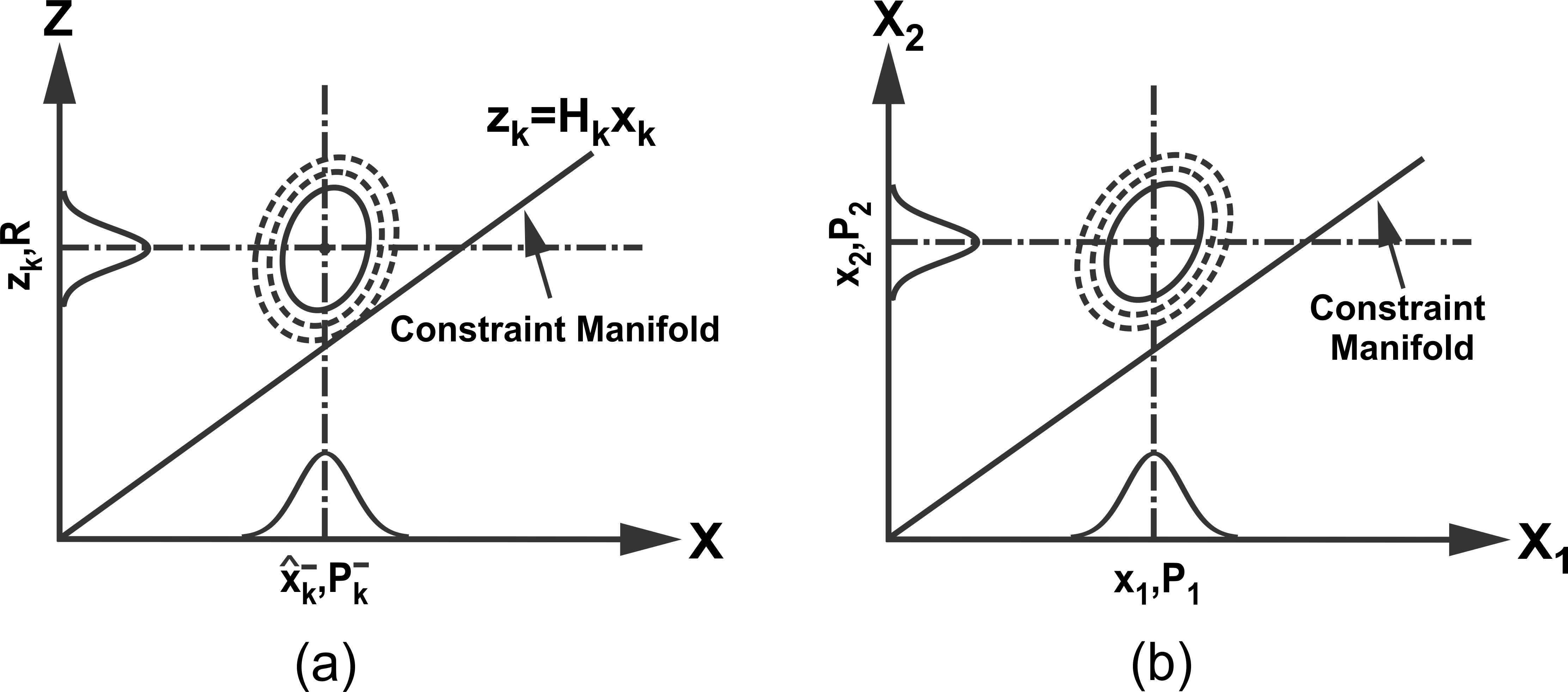 Figure 1. (a) Probability of true states and measurements in the extended space around the data from state predictions and sensor measurements and constraint manifold (b) Extended space representation of two data sources with constraint manifold.
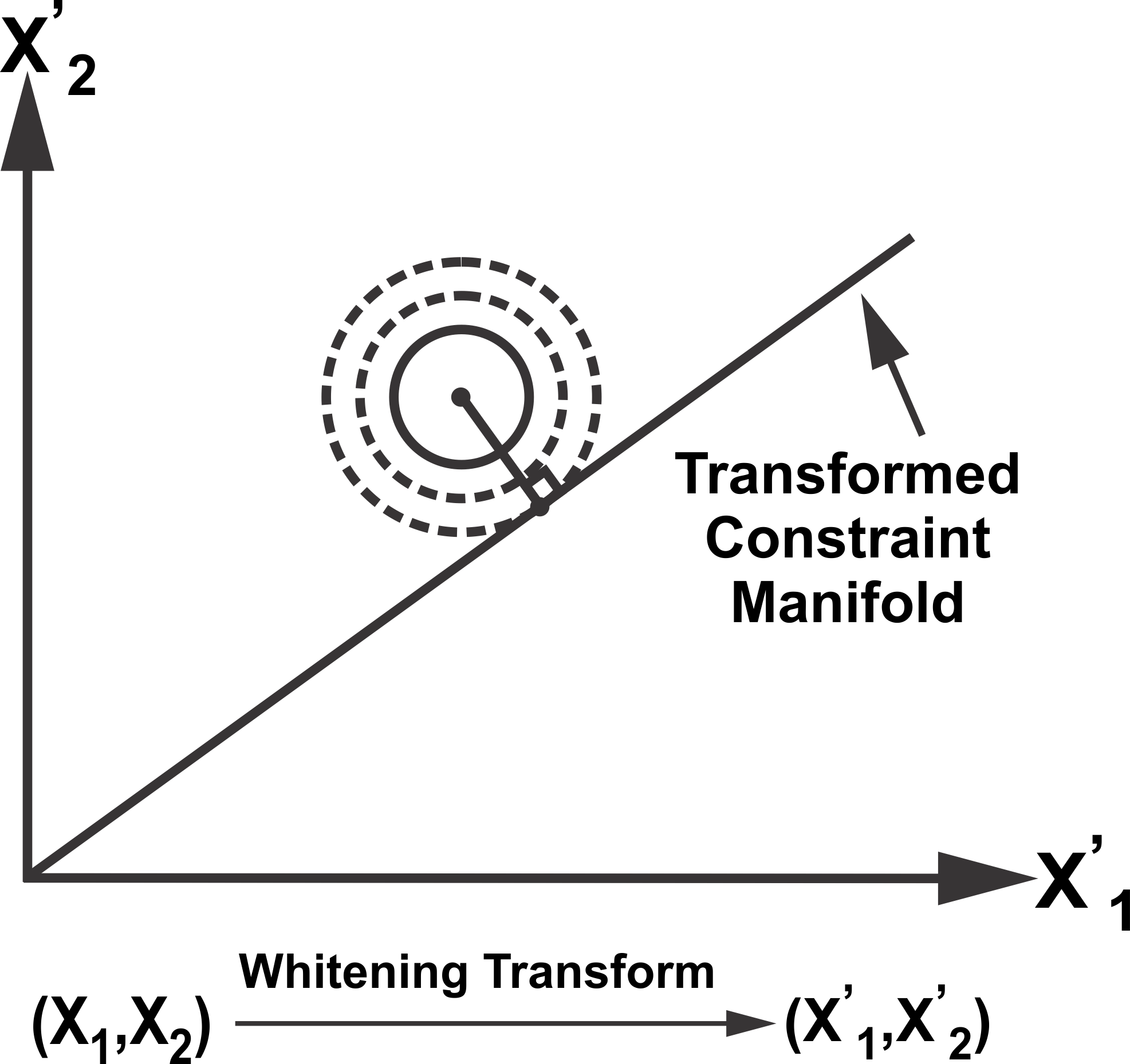
Figure 2. Whitening transform and projection.
To find a point on the constraint manifold with minimum weighted distance, we apply the whitening transform (WT) defined as,  , where
  and
and  are the eigenvalue and eigenvector matrices of
  . Applying WT,
 |
where the matrix  is the subspace of the constraint manifold. Figure 2 illustrates the transformation of the probability distribution as an ellipsoid into a unit circle after WT. The probability distribution is then orthogonally projected on the transformed manifold
  to satisfy the constraints between the data sources in the transformed space as illustrated in Figure 2. Inverse WT is applied to obtain the fused mean estimate and covariance in the original space,
 |
(2) |
 |
(3) |
where  is the orthogonal projection matrix. Using the definition of various components in (2) and (3), a close form simplification can be obtained as,
 |
(4) |
 |
(5) |
Due to the projection in extended space of  , (4) and (5) provide a fused result with respect to each data source. In the case where
  and
and  estimate the same entity, that is,
  , the fused result will be same for the two data sources. As such, a close form equation for fusing redundant data sources in
  can be obtained from (4) and (5) as,
 |
(6) |
 |
(7) |
Given  mean estimates
  of a state
  ∈
∈ with their respective covariances
  ∈
∈  and known cross-covariances
  , (6) and (7) can be used to obtain the optimal fused mean estimate and covariance with
  .
.
For fusing correlated estimates from  redundant sources, the CPF is equivalent to the weighted fusion algorithms [3][4], which compute the fused mean estimate and covariance as a summation of weighted individual estimates as,
 , , |
 |
(8) |
with  . Equivalently, the CP fused mean and covariance can be written as,
 , , |
 |
(9) |
where  and
and  . In the particular case of two data sources, the CP fused solution reduces to the well-known Bar-Shalom Campo formula [5],
 |
(10) |
 |
(11) |
Although equivalent to the traditional approaches in fusing redundant data sources, the proposed method offers a generalized framework not only for fusing correlated data sources but also for handling linear constraints and data inconsistency simultaneously within the framework.
2. Detection of Data Inconsistency
The proposed approach exploits the constraint manifold among sensor estimates to identify any data inconsistency. The identification of inconsistent data is based on the distance from the constraint manifold to the mean of redundant data sources in the extended space that provides a confidence measure with the relative disparity among data sources. Assuming a joint multivariate normal distribution for the data sources, the data confidence can be measured by computing the distance from the constraint manifold as illustrated in Figure 3.
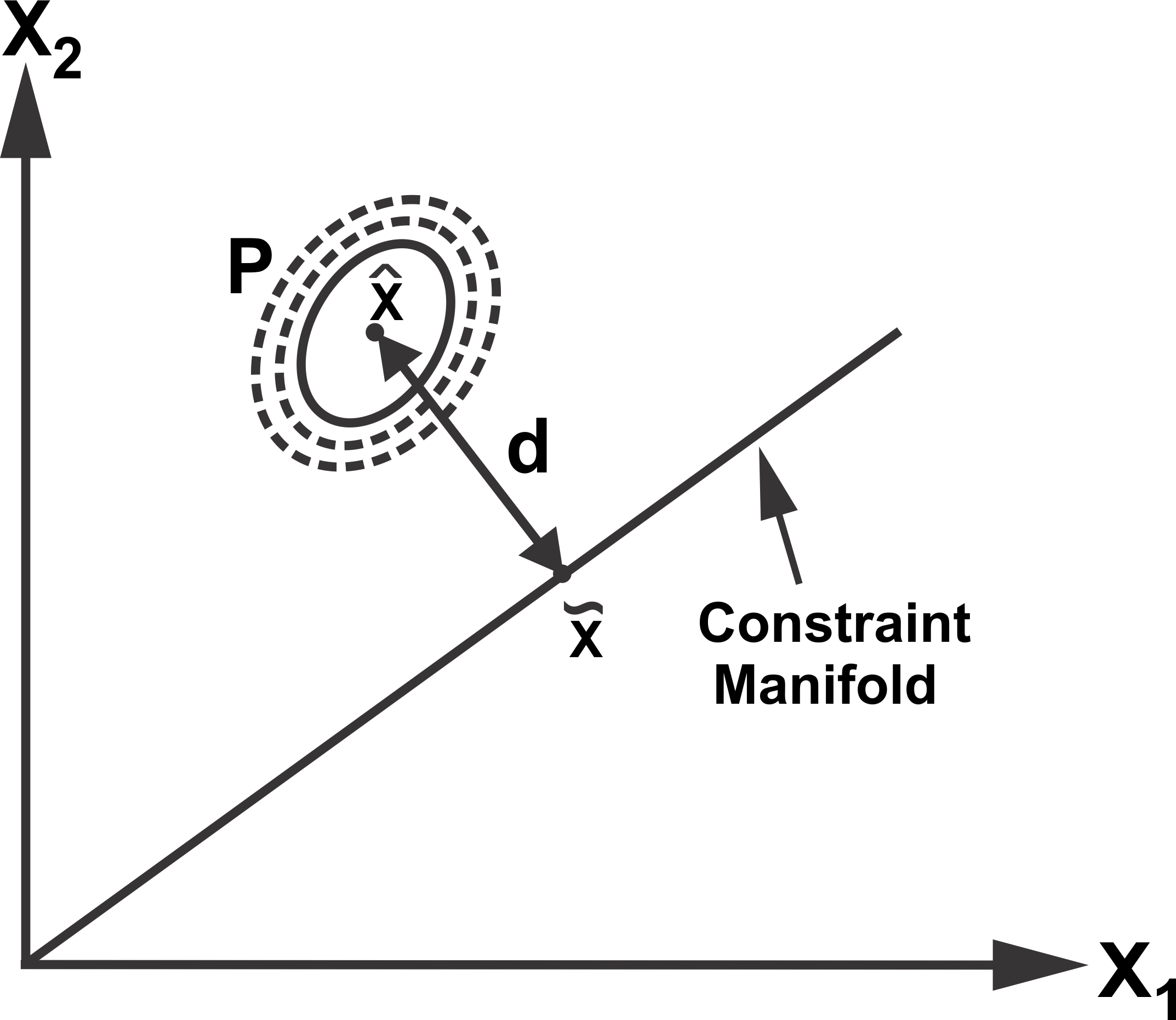 Figure 3. The distance of the multi-variate distribution from the constraint manifold.
Consider the joint space representation of  sensor estimates ,

where  is the dimension of the state vector. The distance
  can be computed as,
 |
(12) |
where  is the point on the manifold and can be obtain by using (4). The
  distance follows a chi-square distribution with
  degrees of freedom (DOF), that is,
  ∼χ2(N0). A chi-square table is then used to obtain the critical value for a particular significance level and DOF. A computed distance
  less than the critical value mean that we are confident about the closeness of sensor estimates and that they can be fused together to provide a better estimate of the underlying states. On the other hand, a distance
  greater than or equal to the critical value indicate spuriousness of the sensor estimates.
3. Incorporation of Linear Constraints
Consider a linear dynamic system model,
 |
(13) |
 |
(14) |
where  represents the discrete-time index,
  is the system matrix,
  is the input matrix,
  is the input vector and
  is the state vector. The system process noise
  with covariance matrix
  and measurement noise
  with covariance
  are assumed to be correlated with cross-covariance
  . The state ∈
 is known to be constrained as,
 |
(15) |
For  ≠ 0, the state space can be translated by a factor such that
  . After constrained state estimation, the state space can be translated back by the factor c to satisfy
  . Hence, without loss of generality, the
  case is considered for analysis here. The matrix
  ∈
∈ is assumed to have a full row rank.
The CPF incorporates any linear constraints among states without any additional processing. Let us denote the constrained filtered estimate of the CPF as  . Assume
  as the predicted state estimate based on the underlying system equation. The extended space representation of the state predictions and measurements of multiple sensors can be written as,
Then the CPF estimate in the presence of linear constraints among states can be obtained using (4) and (5) as,
 |
(16) |
 |
(17) |
where the  matrix is the subspace of the constraint among the state prediction
  and sensor measurements
  as well as linear constraints
  among state variables. The subspace of the linear constraint among state prediction and sensor measurements can be written as,

Then,  is a combination of
  and
and  , that is,
 ∈
∈
The projection of the probability distribution of true states and measurements around the predicted states and actual measurements onto the constraint manifold  in the extended space provide the filtered or fused estimate of state prediction and sensor measurements as well as completely satisfying the linear constraints among the states directly in one step.
References
- Muhammad Abu Bakr and Sukhan Lee A framework of covariance projection on constraint manifold for data fusion. Sensors 2018, 18, 1610, https://doi.org/10.3390/s18051610.
- Muhammad Abu Bakr and Sukhan Lee, “A general framework for data fusion and outlier removal in distributed sensor networks,” in IEEE International Conference on Multisensor Fusion and Integration for Intelligent Systems, 2017.
- Vladimir Shin, Younghee Lee and Tae-Sun Choi Generalized Millman’s formula and its application for estimation problems. Signal Processing 2006, 86, 257-266, https://doi.org/10.1016/j.sigpro.2005.05.015.
- Shu-li Sun Multi-sensor optimal information fusion Kalman filters with applications. Aerospace Science and Technology 2004, 8, 57-62, https://doi.org/10.1016/j.ast.2003.08.003.
- Yaahov Bar-Shalom and Leon Campo The effect of the common process noise on the two-sensor fused-track covariance. IEEE Transactions on Aerospace and Electronic Systems 1986, 6, 803-805, 10.1109/TAES.1986.310815.

