Your browser does not fully support modern features. Please upgrade for a smoother experience.
Submitted Successfully!
 +1 credit
Thank you for your contribution! You can also upload a video entry or images related to this topic.
For video creation, please contact our Academic Video Service.
| Version | Summary | Created by | Modification | Content Size | Created at | Operation |
|---|---|---|---|---|---|---|
| 1 | Hamed Rezapour | -- | 2283 | 2023-06-21 09:46:28 | | | |
| 2 | Camila Xu | Meta information modification | 2283 | 2023-06-21 10:20:21 | | | | |
| 3 | Camila Xu | Meta information modification | 2283 | 2023-06-21 10:22:53 | | | | |
| 4 | Camila Xu | Meta information modification | 2248 | 2023-06-26 10:14:39 | | |
Video Upload Options
We provide professional Academic Video Service to translate complex research into visually appealing presentations. Would you like to try it?
Cite
If you have any further questions, please contact Encyclopedia Editorial Office.
Rezapour, H.; Jamali, S.; Bahmanyar, A. Artificial Intelligence-Based Methods in Power Distribution Networks. Encyclopedia. Available online: https://encyclopedia.pub/entry/45908 (accessed on 25 July 2026).
Rezapour H, Jamali S, Bahmanyar A. Artificial Intelligence-Based Methods in Power Distribution Networks. Encyclopedia. Available at: https://encyclopedia.pub/entry/45908. Accessed July 25, 2026.
Rezapour, Hamed, Sadegh Jamali, Alireza Bahmanyar. "Artificial Intelligence-Based Methods in Power Distribution Networks" Encyclopedia, https://encyclopedia.pub/entry/45908 (accessed July 25, 2026).
Rezapour, H., Jamali, S., & Bahmanyar, A. (2023, June 21). Artificial Intelligence-Based Methods in Power Distribution Networks. In Encyclopedia. https://encyclopedia.pub/entry/45908
Rezapour, Hamed, et al. "Artificial Intelligence-Based Methods in Power Distribution Networks." Encyclopedia. Web. 21 June, 2023.
Copy Citation
Following to a short-circuit fault in distribution networks, the fault should be located and isolated before restoring the supply. A fast and accurate fault location method can help to improve the continuity of supply considerably. In general, the distribution-network fault location methods can be categorized into impedance-based methods, state estimation-based methods, traveling wave-based methods, and artificial intelligence-based (AI-based) methods.
fault location
artificial intelligence
power distribution networks
1. Introduction
Following to a short-circuit fault in distribution networks, the fault should be located and isolated before restoring the supply. A fast and accurate fault location method can help to improve the continuity of supply considerably. In general, the distribution-network fault location methods can be categorized into impedance-based methods, state estimation-based methods, traveling wave-based methods, and artificial intelligence-based (AI-based) methods.
The impedance-based methods determine the location of faults by measuring the apparent impedance seen from one or more measurement points. These methods estimate the fault location by comparing the measured impedance for the probable fault paths in the network with the measured one [1][2][3][4][5]. These methods can provide fault location estimations with acceptable accuracy, although they might estimate several candidate locations in the networks with several laterals. They require detailed data about the network topology, line impedances, and loads and are, hence, very sensitive to network-model inaccuracies.
State estimation-based methods consider a fault as bad data and try to locate it using the data collected from different measurement points of the network [6][7][8]. Similar to the impedance-based methods, these techniques need the distribution-network data. While they are less sensitive to input data inaccuracies, they can only be applied to networks with considerable measurement infrastructures.
Traveling wave-based methods estimate the fault location by calculating the sweep duration of the wave traveling from the measurement point to the fault location [9][10][11][12]. These methods are practically applicable to long transmission lines. However, their application to distribution networks with short line sections demands very high measurement sampling frequency which is not practical. Moreover, the application of these methods to networks with various laterals is challenging.
AI-based methods can be trained in off-line procedures to make fast online estimations of the fault location or faulted section. These methods need a considerable amount of training data which can be based on historical records or be generated in a simulation process.
AI-based algorithms are widely used in various fault diagnosis applications. In [13], an artificial neural network (ANN) based on ACO-DWT is developed for fault identification and classification in HVDC networks. In [14], a method combining attention mechanism and long short-term memory (LSTM) is proposed to investigate tool condition monitoring in milling applications. A tangent hyperbolic fuzzy entropy measure-based method for determining the most sensitive frequency band to easily identify defective components in an axial piston pump is proposed by [15].
2. AI-Based Methods
The application process of AI-based methods is illustrated in Figure 1. The first step of applications is to choose the input variables which comprehend the network condition. In the second step, the features of voltage or current are adopted by using transforms such as Wavelet, Stockwell, and Fast Fourier to generate informative features. Some features are based on high-frequency spectra of signals, and some are based on the fundamental frequency spectrum of the signal such as the root mean square (RMS) value of the fundamental signal. Finally, in the last step, the main algorithm analyzes the input features and gives an estimation of the fault location as the output. In the following, some of the main algorithms employed by the AI-based fault location methods are discussed in details and discussions about each of these steps are provided in their corresponding sections.

Figure 1. The process of AI-based fault location methods.
2.1. Artificial Neural Networks (ANNs)
ANN is the most used AI-based algorithm in the field of fault location due to its flexibility and high precision [10][16][17][18][19][20][21][22][23][24][25][26][27][28][29][30][31][32][33][34][35][36][37]. ANNs are a class of supervised regression algorithms that can be used as a prediction tool. The training procedure of ANNs is based on a series of experienced samples of the system. In a fault location method, the training samples are formed of tuples including inputs (e.g., current or voltage features) and outputs (e.g., fault distance or fault reactance). The training data is often adopted from simulations because this data is extracted from the fault condition, and it is not possible to apply several faults on real-world systems to generate data. However, there might be a record of previous fault signals; ANN needs a large amount of data in different network conditions and fault situations, and the recorded data are often insufficient.
An ANN is simply constructed of different layers. There are three types of layers in ANNs: the first as the input layer, the last as the output layer, and hidden layers in between. The input layer connects the input variables (features) to the neurons in the first hidden layer. The hidden layers construct a network connection from the input layer to the output layer and the output layer contains a number of neurons (equal to the number of outputs) connected to the last hidden layer. Figure 2 shows a typical example of an ANN.

Figure 2. A typical ANN showing network layers connection.
In an ANN, each neuron acts based on its activation function as Equation (1):
where 𝑦, 𝑥, and 𝑤 are the output, input, and corresponding weights of the neuron.
The activation function is dependent on the type of the ANN and most papers proposed hyperbolic tangent. The number of hidden layers and the number of neurons in each hidden layer is modified based on the experience of the designer depending on the size and complexity of the problem. After determining the type of the network and the number of neurons, the weights should be determined within a training process [38].
There are different methods to calculate the optimized weights; Levenberg–Marquardt, backpropagation, and evolutionary algorithms (GA, PSO, ACO, etc.) are examples of these methods.
In addition to the fully connected ANNs, there are other novel neural networks such as conventional neural networks (CNNs) and recurrent neural networks (RNNs). The key components of a CNN include convolutional layers, pooling layers, and fully connected layers (basic ANN). In the convolutional layers, the network applies a set of filters to the input sample, producing a set of feature maps that highlight different aspects of the sample. The pooling layers downsample the feature maps, reducing their dimensionality and creating a more compact representation of the image. Finally, the fully connected layers use the features extracted by the convolutional and pooling layers to make predictions or classifications [27][39][40][41]. In fault location applications, first, a signal-to-image transform is performed to create images from recorded fault data appropriate for the convolutional process, and, then, the exact fault location is investigated by the fully connected ANN [42][43].
RNNs are a type of neural network that are designed to work with sequential data. Unlike fully connected neural networks that process inputs in a single pass, RNNs process inputs in a sequential manner, while also maintaining a hidden state that captures information from previous inputs. The key feature of RNNs is their ability to capture and learn temporal dependencies in sequential data. This is achieved by using recurrent connections that allow the network to pass information from one time step to the next. The hidden state of the network at each time step is a function of the current input and the previous hidden state, allowing the network to maintain a memory of past inputs [44][45][46].
2.2. Support Vector Machine (SVM)
SVM is a powerful tool for handling classification and regression problems [16]. This method determines hyperplanes for separating different classes. For example, in a two-dimension two-class problem, the SVM method determines the line separating the classes, as shown in Figure 3 [47][48].

Figure 3. SVM method applied to a simple two-dimension two-class problem.
For more complex systems, SVM adds an extra feature to the samples (maps the problem into a higher dimensional space) and proposes a hyperplane in the D-dimensional space [49]. In fault location applications, SVM is used as a regression tool to estimate the output value (fault location here). While SVM is a tool for linear systems, however, it can be applied to nonlinear problems using the kernel trick [24]. SVM maps inputs to outputs using the following equation:
where 𝑦 is the output, 𝑥 is the input, is the weight vector and

is the basis function.
To solve the problem, a loss function is defined as below.
where 𝜀 is a threshold for the loss function and 𝛽 is the target value of the training sample 𝑥. Minimizing Equation (4) is the main task of the SVM can be handled using different optimization methods.
where 𝑁 is the number of the training samples.
2.3. K-Nearest Neighbor
KNN is a simple supervised machine-learning algorithm for both objectives of regression and classification. In fault location applications, KNN is used for both classification and regression purposes, faulted line section and fault type detection are of the classification applications, and determination of fault location is of the regression applications [50][51]. In this method, the test sample is assigned to the nearest classes depending on the value of K, e.g., if K equals to 1, the sample will be assigned to the first nearest neighbor and if the K equals to 3, the sample will be assigned to the class that is more repeated in the three closest neighbors. Figure 4 shows an example to assign a sample (green square) into two classes; if k equals to 1 (dashed red circle) the sample assigns to class 2 (blue triangles) and if k equals to 3, (solid red circle) the sample assigns to class 1 (orange circles). In some applications, the sample is assigned using weights based on the distance of the sample to the class samples.
Figure 4. A typical example of the KNN classification method (the green square is the test data, and the red line shows the neighboring area).
The main disadvantage of KNN is its slow response in high-dimension problems. To overcome this issue, the research used KNN in conjunction with ANNs [23][33]. In these methods, KNN processes the outputs of ANN to improve efficiency and the precision of ANN. Furthermore, this technique reduces the number of KNN input variables that are independent of the network structure and size.
2.4. Deep Reinforcement Learning
Deep learning is inspired by the evolution of mammals’ brains. In this method, an agent is trained based on its experiences where actions with rewards registered as good choices and actions with harm registered as unfavorable choices and the agent chooses its next action trying to maximize its reward. Favorable or unfavorable conditions are determined depending on the agent and the environment, e.g., for a mammal, finding food is a favorable situation, and falling from a cliff is unfavorable. In optimization or classification applications, favorability is determined by the operator. For example, for a can gatherer robot, finding new cans is a situation with pleasure, and losing battery is not encouraging.
The fundamentals of deep learning are based on reinforcement Q-learning. Q-learning is an efficient optimization tool for solving multistage problems. In each stage of the problem, the next stage (state) is a function of the present stage and the chosen action is based on the following:
where 𝑥𝑘 is the present state, 𝑎𝑘 is the chosen action, and 𝑥𝑘+1 is the next state.
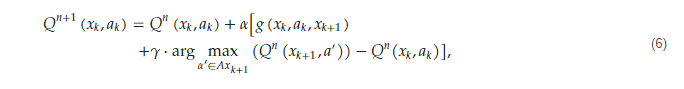
In this method, each state-action tuple (𝑥𝑘,𝑎𝑘)has a related Q-value and the agent in each state chooses the action with maximum Q-value and reaches the next state. The Q-values are in relation to rewards or penalties the agent gained during its training process (experiences). Q-value for each state action is dependent on its immediate reward and those it might gain in the following next states based on the following equation:
where 𝑛 is the number of the training iteration, is the immediate reward, 𝛼 is the training rate, and 𝛾 is the discount factor. is dependent to the situation of the next state representing what the agent will experience.
Due to the curse of dimensionality, determining is not an easy job in high dimension or continuous problems and needs high calculation efforts. To cope with this problem, deep neural networks are hired as a regression tool to estimate for each state-action tuple. The training procedure of DNNs can be performed by using batch-constrained sets of data, including agent experiences, that simulate the behavior of the agent and responses of the environment.
In fault location applications, the agent should be able to classify the fault type and determine the fault location. Hence, the agent should be trained as a tool for regression and classification applications. The input variables can be voltage or current features and the output variables are fault type (e.g., the line to ground (LG), line to line (LL), line to line to ground (LLG), three phase (LLL)), and fault location (a continuous value).
In [52], the authors developed a deep neural network-based (DNN-based) method for fault location and identification in low-voltage grids that is topology independent and can also localize high-impedance faults. In [28], the authors presented a DRL algorithm for fault diagnosis applications that is goal-oriented and independent of a large amount of labelled data.
References
- Krishnathevar, R.; Ngu, E.E. Generalized Impedance-Based Fault Location for Distribution Systems. IEEE Trans. Power Deliv. 2012, 27, 449–451.
- Salim, R.H.; Salim, K.C.O.; Bretas, A.S. Further Improvements on Impedance-Based Fault Location for Power Distribution Systems. IET Gener. Transm. Distrib. 2011, 5, 467–478.
- Gabr, M.A.; Ibrahim, D.K.; Ahmed, E.S.; Gilany, M.I. A New Impedance-Based Fault Location Scheme for Overhead Unbalanced Radial Distribution Networks. Electr. Power Syst. Res. 2017, 142, 153–162.
- Ferreira, G.D.; Gazzana, D.S.; Bretas, A.S.; Netto, A.S. A Unified Impedance-Based Fault Location Method for Generalized Distribution Systems. In Proceedings of the 2012 IEEE Power and Energy Society General Meeting, San Diego, CA, USA, 22–26 July 2012.
- Personal, E.; García, A.; Parejo, A.; Larios, D.F.; Biscarri, F.; León, C. A Comparison of Impedance-Based Fault Location Methods for Power Underground Distribution Systems. Energies 2016, 9, 1022.
- Usman, M.U.; Omar Faruque, M. Validation of a PMU-Based Fault Location Identification Method for Smart Distribution Network with Photovoltaics Using Real-Time Data. IET Gener. Transm. Distrib. 2018, 12, 5824–5833.
- Gholami, M.; Abbaspour, A.; Moeini-Aghtaie, M.; Fotuhi-Firuzabad, M.; Lehtonen, M. Detecting the Location of Short-Circuit Faults in Active Distribution Network Using PMU-Based State Estimation. IEEE Trans. Smart Grid 2020, 11, 1396–1406.
- Jamali, S.; Bahmanyar, A.; Bompard, E. Fault Location Method for Distribution Networks Using Smart Meters. Measurement 2017, 102, 150–157.
- Xie, L.; Luo, L.; Li, Y.; Zhang, Y.; Cao, Y. A Traveling Wave-Based Fault Location Method Employing VMD-TEO for Distribution Network. IEEE Trans. Power Deliv. 2020, 35, 1987–1998.
- Pourahmadi-Nakhli, M.; Safavi, A.A. Path Characteristic Frequency-Based Fault Locating in Radial Distribution Systems Using Wavelets and Neural Networks. IEEE Trans. Power Deliv. 2011, 26, 772–781.
- Chen, R.; Yin, X.; Yin, X.; Li, Y.; Lin, J. Computational Fault Time Difference-Based Fault Location Method for Branched Power Distribution Networks. IEEE Access 2019, 7, 181972–181982.
- Jianwen, Z.; Hui, H.; Yu, G.; Yongping, H.; Shuping, G.; Jianan, L. Single-Phase Ground Fault Location Method for Distribution Network Based on Traveling Wave Time-Frequency Characteristics. Electr. Power Syst. Res. 2020, 186, 106401.
- Jawad, R.S.; Abid, H. HVDC Fault Detection and Classification with Artificial Neural Network Based on ACO-DWT Method. Energies 2023, 16, 1064.
- Zheng, G.; Chen, W.; Qian, Q.; Kumar, A.; Sun, W.; Zhou, Y. TCM in Milling Processes Based on Attention Mechanism-Combined Long Short-Term Memory Using a Sound Sensor under Different Working Conditions. Int. J. Hydromechatron. 2022, 5, 243–259.
- Zhou, Y.; Kumar, A.; Parkash, C.; Vashishtha, G.; Tang, H.; Glocawz, A.; Dong, A.; Xiang, J. Development of Entropy Measure for Selecting Highly Sensitive WPT Band to Identify Defective Components of an Axial Piston Pump. Appl. Acoust. 2023, 203, 109225.
- Thukaram, D.; Khincha, H.P.; Vijaynarasimha, H.P. Artificial Neural Network and Support Vector Machine Approach for Locating Faults in Radial Distribution Systems. IEEE Trans. Power Deliv. 2005, 20, 710–721.
- Rafinia, A.; Moshtagh, J. A New Approach to Fault Location in Three-Phase Underground Distribution System Using Combination of Wavelet Analysis with ANN and FLS. Int. J. Electr. Power Energy Syst. 2014, 55, 261–274.
- Chen, X.; Yin, X.; Deng, S. A Novel Method for SLG Fault Location in Power Distribution System Using Time Lag of Travelling Wave Components. IEEJ Trans. Electr. Electron. Eng. 2017, 12, 45–54.
- Dashtdar, M.; Dashti, R.; Shaker, H.R. Distribution Network Fault Section Identification and Fault Location Using Artificial Neural Network. In Proceedings of the 2018 5th International Conference on Electrical and Electronic Engineering (ICEEE), Istanbul, Turkey, 3–5 May 2018; pp. 273–278.
- Chunju, F.; Li, K.K.; Chan, W.L.; Weiyong, Y.; Zhaoning, Z. Application of Wavelet Fuzzy Neural Network in Locating Single Line to Ground Fault (SLG) in Distribution Lines. Int. J. Electr. Power Energy Syst. 2007, 29, 497–503.
- Aslan, Y.; Yağan, Y.E. Artificial Neural-Network-Based Fault Location for Power Distribution Lines Using the Frequency Spectra of Fault Data. Electr. Eng. 2017, 99, 301–311.
- Javadian, S.A.M.; Nasrabadi, A.M.; Haghifam, M.R.; Rezvantalab, J. Determining Fault’s Type and Accurate Location in Distribution Systems with DG Using MLP Neural Networks. In Proceedings of the 2009 International Conference on Clean Electrical Power, ICCEP 2009, Capri, Italy, 9–11 June 2009; pp. 284–289.
- Jamali, S.; Ranjbar, S.; Bahmanyar, A. Identification of Faulted Line Section in Microgrids Using Data Mining Method Based on Feature Discretisation. Int. Trans. Electr. Energy Syst. 2020, 30, e12353.
- Lin, H.; Sun, K.; Tan, Z.H.; Liu, C.; Guerrero, J.M.; Vasquez, J.C. Adaptive Protection Combined with Machine Learning for Microgrids. IET Gener. Transm. Distrib. 2019, 13, 770–779.
- Bakkar, M.; Bogarra, S.; Córcoles, F.; Aboelhassan, A.; Wang, S.; Iglesias, J. Artificial Intelligence-Based Protection for Smart Grids. Energies 2022, 15, 4933.
- Usman, M.U.; Ospina, J.; Faruque, M.O. Fault Classification and Location Identification in a Smart Distribution Network Using ANN. In Proceedings of the 2018 IEEE Power & Energy Society General Meeting (PESGM), Portland, OR, USA, 5–10 August 2018.
- Chen, K.; Hu, J.; Zhang, Y.; Yu, Z.; He, J. Fault Location in Power Distribution Systems via Deep Graph Convolutional Networks. IEEE J. Sel. Areas Commun. 2020, 38, 119–131.
- Li, M.; Zhang, H.; Ji, T.; Wu, Q.H. Fault Identification in Power Network Based on Deep Reinforcement Learning. CSEE J. Power Energy Syst. 2022, 8, 721–731.
- Shafiullah, M.; Abido, M.A.; Al-Hamouz, Z. Wavelet-Based Extreme Learning Machine for Distribution Grid Fault Location. IET Gener. Transm. Distrib. 2017, 11, 4256–4263.
- Lout, K.; Aggarwal, R.K. Current Transients Based Phase Selection and Fault Location in Active Distribution Networks with Spurs Using Artificial Intelligence. In Proceedings of the 2013 IEEE Power & Energy Society General Meeting, Vancouver, BC, Canada, 21–25 July 2013.
- Ray, P.; Mishra, D. Artificial Intelligence Based Fault Location in a Distribution System. In Proceedings of the 2014 International Conference on Information Technology, ICIT 2014, Bhubaneswar, India, 22–24 December 2014; pp. 18–23.
- Barra, P.H.A.; Pessoa, A.L.D.S.; Menezes, T.S.; Santos, G.G.; Coury, D.V.; Oleskovicz, M. Fault Location in Radial Distribution Networks Using ANN and Superimposed Components. In Proceedings of the 2019 IEEE PES Innovative Smart Grid Technologies Conference-Latin America (ISGT Latin America), Gramado, Brazil, 15–18 September 2019.
- Jamali, S.; Bahmanyar, A.; Ranjbar, S. Hybrid Classifier for Fault Location in Active Distribution Networks. Prot. Control Mod. Power Syst. 2020, 5, 17.
- Dehghani, F.; Nezami, H. A New Fault Location Technique on Radial Distribution Systems Using Artificial Neural Network. IET Conf. Publ. 2013, 2013, 13712520.
- Aslan, Y. An Alternative Approach to Fault Location on Power Distribution Feeders with Embedded Remote-End Power Generation Using Artificial Neural Networks. Electr. Eng. 2012, 94, 125–134.
- Aslan, Y.; Yagan, Y.E. ANN Based Fault Location for Medium Voltage Distribution Lines with Remote-End Source. In Proceedings of the 2016 International Symposium on Fundamentals of Electrical Engineering (ISFEE), Bucharest, Romania, 30 June–2 July 2016.
- Mohamed, E.A.; Rao, N.D. Artificial Neural Network Based Fault Diagnostic System for Electric Power Distribution Feeders. Electr. Power Syst. Res. 1995, 35, 1–10.
- Kenji, S. Artificial Neural Networks-Architectures and Applications; BoD–Books on Demand: Norderstedt, Germany, 2013; ISBN 9535109359.
- O’Shea, K.; Nash, R. An Introduction to Convolutional Neural Networks. Int. J. Res. Appl. Sci. Eng. Technol. 2015, 10, 943–947.
- Gu, J.; Wang, Z.; Kuen, J.; Ma, L.; Shahroudy, A.; Shuai, B.; Liu, T.; Wang, X.; Wang, G.; Cai, J.; et al. Recent Advances in Convolutional Neural Networks. Pattern Recognit. 2018, 77, 354–377.
- Li, Z.; Liu, F.; Yang, W.; Peng, S.; Zhou, J. A Survey of Convolutional Neural Networks: Analysis, Applications, and Prospects. IEEE Trans. Neural Netw. Learn. Syst. 2022, 33, 6999–7019.
- Yu, Y.; Li, M.; Ji, T.; Wu, Q.H. Fault Location in Distribution System Using Convolutional Neural Network Based on Domain Transformation. CSEE J. Power Energy Syst. 2021, 7, 472–484.
- Shi, X.; Xu, Y. A Fault Location Method for Distribution System Based on One-Dimensional Convolutional Neural Network. In Proceedings of the 2021 IEEE International Conference on Power, Intelligent Computing and Systems (ICPICS), Shenyang, China, 29–31 July 2021; pp. 333–337.
- Salehinejad, H.; Sankar, S.; Barfett, J.; Colak, E.; Valaee, S. Recent Advances in Recurrent Neural Networks. arXiv 2017, arXiv:1801.01078.
- Lin, F.; Zhang, Y.; Wang, K.; Wang, J.; Zhu, M. Parametric Probabilistic Forecasting of Solar Power with Fat-Tailed Distributions and Deep Neural Networks. IEEE Trans. Sustain. Energy 2022, 13, 2133–2147.
- Wang, K.; Zhang, Y.; Lin, F.; Wang, J.; Zhu, M. Nonparametric Probabilistic Forecasting for Wind Power Generation Using Quadratic Spline Quantile Function and Autoregressive Recurrent Neural Network. IEEE Trans. Sustain. Energy 2022, 13, 1930–1943.
- Ripley, B.D. Neural Networks and Related Methods for Classification. J. R. Stat. Soc. Ser. B Stat. Methodol. 1994, 56, 409–437.
- Kaufman, L. Solving the Quadratic Programming Problem Arising in Support Vector Classification. In Advances in Kernel Methods; MIT Press: Cambridge, MA, USA, 2022; pp. 147–167.
- Salat, R.; Osowski, S. Accurate Fault Location in the Power Transmission Line Using Support Vector Machine Approach. IEEE Trans. Power Syst. 2004, 19, 979–986.
- Manohar, M.; Koley, E.; Ghosh, S. Reliable Protection Scheme for PV Integrated Microgrid Using an Ensemble Classifier Approach with Real-Time Validation. IET Sci. Meas. Technol. 2018, 12, 200–208.
- Majidi, M.; Etezadi-Amoli, M.; Fadali, M.S. A Novel Method for Single and Simultaneous Fault Location in Distribution Networks. IEEE Trans. Power Syst. 2015, 30, 3368–3376.
- Sapountzoglou, N.; Lago, J.; De Schutter, B.; Raison, B. A Generalizable and Sensor-Independent Deep Learning Method for Fault Detection and Location in Low-Voltage Distribution Grids. Appl. Energy 2020, 276, 115299.
More
Information
Subjects:
Engineering, Electrical & Electronic
Contributors
MDPI registered users' name will be linked to their SciProfiles pages. To register with us, please refer to https://encyclopedia.pub/register
:
View Times:
1.0K
Revisions:
4 times
(View History)
Update Date:
26 Jun 2023
Table of Contents


Notice
You are not a member of the advisory board for this topic. If you want to update advisory board member profile, please contact office@encyclopedia.pub.
OK
Confirm
Only members of the Encyclopedia advisory board for this topic are allowed to note entries. Would you like to become an advisory board member of the Encyclopedia?
Yes
No
${ textCharacter }/${ maxCharacter }
Submit
Cancel
Back
Comments
${ item }
|
${ item.createdUser.fullName }
${ item.createdAt }
${ item.vote }
${ item.reply }
Delete
${ reply.createdUser.fullName }
${ reply.createdAt }
${ reply.vote }
Delete
There is no reply to this comment~
${ item.replyTextCharacter }/${ item.replyMaxCharacter }
Submit
Cancel
More
No more~
There is no comment~
${ textCharacter }/${ maxCharacter }
Submit
Cancel
${ selectedItem.replyTextCharacter }/${ selectedItem.replyMaxCharacter }
Submit
Cancel
Confirm
Are you sure to Delete?
Yes
No