1. Decimation by an Integer Factor

Decimation by an integer factor, M, can be explained as a two-step process, with an equivalent implementation that is more efficient:

1. Reduce high-frequency signal components with a digital lowpass filter.
2. Downsample the filtered signal by M; that is, keep only every M^th sample.

Downsampling alone causes high-frequency signal components to be misinterpreted by subsequent users of the data, which is a form of distortion called aliasing. The first step, if necessary, is to suppress aliasing to an acceptable level. In this application, the filter is called an anti-aliasing filter, and its design is discussed below. Also see undersampling for information about downsampling bandpass functions and signals.

When the anti-aliasing filter is an IIR design, it relies on feedback from output to input, prior to the downsampling step. With FIR filtering, it is an easy matter to compute only every M^th output. The calculation performed by a decimating FIR filter for the n^th output sample is a dot product:

[math]\displaystyle{ y[n] = \sum_{k=0}^{K-1} x[nM-k]\cdot h[k], }[/math]

where the h[•] sequence is the impulse response, and K is its length.  x[•] represents the input sequence being downsampled. In a general purpose processor, after computing y[n], the easiest way to compute y[n+1] is to advance the starting index in the x[•] array by M, and recompute the dot product. In the case M=2, h[•] can be designed as a half-band filter, where almost half of the coefficients are zero and need not be included in the dot products.

Impulse response coefficients taken at intervals of M form a subsequence, and there are M such subsequences (phases) multiplexed together. The dot product is the sum of the dot products of each subsequence with the corresponding samples of the x[•] sequence. Furthermore, because of downsampling by M, the stream of x[•] samples involved in any one of the M dot products is never involved in the other dot products. Thus M low-order FIR filters are each filtering one of M multiplexed phases of the input stream, and the M outputs are being summed. This viewpoint offers a different implementation that might be advantageous in a multi-processor architecture. In other words, the input stream is demultiplexed and sent through a bank of M filters whose outputs are summed. When implemented that way, it is called a polyphase filter.

For completeness, we now mention that a possible, but unlikely, implementation of each phase is to replace the coefficients of the other phases with zeros in a copy of the h[•] array, process the original x[•] sequence at the input rate, and decimate the output by a factor of M. The equivalence of this inefficient method and the implementation described above is known as the first Noble identity.^[1]

1.1. Anti-Aliasing Filter

The requirements of the anti-aliasing filter can be deduced from any of the three pairs of graphs in Fig. 1. Note that all three pairs are identical, except for the units of the abscissa variables. The upper graph of each pair is an example of the periodic frequency distribution of a sampled function, x(t), with Fourier transform, X(f). The lower graph is the new distribution that results when x(t) is sampled three times slower, or (equivalently) when the original sample sequence is decimated by a factor of M=3. In all three cases, the condition that ensures the copies of X(f) do not overlap each other is the same: [math]\displaystyle{ B \lt \tfrac{1}{M}\cdot\tfrac{1}{2T}, }[/math]  where T is the interval between samples, 1/T is the sample-rate, and 1/(2T) is the Nyquist frequency. The anti-aliasing filter that can ensure the condition is met has a cutoff frequency less than [math]\displaystyle{ \tfrac{1}{M} }[/math] times the Nyquist frequency.^[2]

The abscissa of the top pair of graphs represents the discrete-time Fourier transform (DTFT), which is a Fourier series representation of a periodic summation of X(f):

[math]\displaystyle{ \underbrace{ \sum_{n=-\infty}^{\infty} \overbrace{x(nT)}^{x[n]}\ \mathrm e^{-\mathrm i 2\pi f nT} }_{\text{DTFT}} = \frac{1}{T}\sum_{k=-\infty}^{\infty} X\Bigl(f - \frac{k}{T}\Bigr). }[/math]

(Eq.1)

When T has units of seconds, [math]\displaystyle{ \scriptstyle f }[/math] has units of hertz. Replacing T with MT in the formulas above gives the DTFT of the decimated sequence, x[nM]:

[math]\displaystyle{ \sum_{n=-\infty}^{\infty} x(n\cdot MT)\ \mathrm e^{-\mathrm i 2\pi f n(MT)} = \frac{1}{MT}\sum_{k=-\infty}^{\infty} X\left(f-\tfrac{k}{MT}\right). }[/math]

The periodic summation has been reduced in amplitude and periodicity by a factor of M, as depicted in the second graph of Fig. 1.  Aliasing occurs when adjacent copies of X(f) overlap. The purpose of the anti-aliasing filter is to ensure that the reduced periodicity does not create overlap.

In the middle pair of graphs, the frequency variable, [math]\displaystyle{ \scriptstyle f, }[/math] has been replaced by normalized frequency, which creates a periodicity of 1 and a Nyquist frequency of ½. ^[3]  A common practice in filter design programs is to assume those values and request only the corresponding cutoff frequency in the same units. In other words, the cutoff frequency [math]\displaystyle{ B_{max} = \tfrac{1}{M}\cdot\tfrac{1}{2T}, }[/math] is normalized to [math]\displaystyle{ TB_{max} = \tfrac{1}{M}\cdot\tfrac{1}{2} = \tfrac{0.5}{M}. }[/math]   The units of this quantity are (seconds/sample)×(cycles/second) = cycles/sample.

The bottom pair of graphs represent the Z-transforms of the original sequence and the decimated sequence, constrained to values of complex-variable, z, of the form [math]\displaystyle{ z=\mathrm e^{\mathrm i\omega}. }[/math]  Then the transform of the x[n] sequence has the form of a Fourier series. By comparison with Eq.1, we deduce:

[math]\displaystyle{ \sum_{n=-\infty}^{\infty} x[n]\ z^{-n} = \sum_{n=-\infty}^{\infty} x(nT)\ \mathrm e^{-\mathrm i\omega n} = \frac{1}{T}\sum_{k=-\infty}^{\infty} \underbrace{X\Bigl(\tfrac{\omega}{2\pi T} - \tfrac{k}{T}\Bigr)}_{X\Bigl(\frac{\omega - 2\pi k}{2\pi T}\Bigr)}, }[/math]

which is depicted by the fifth graph in Fig. 1.  Similarly, the sixth graph depicts:

[math]\displaystyle{ \sum_{n=-\infty}^{\infty} x[nM]\ z^{-n} = \sum_{n=-\infty}^{\infty} x(nMT)\ \mathrm e^{-\mathrm i\omega n} = \frac{1}{MT}\sum_{k=-\infty}^{\infty} \underbrace{X\Bigl(\tfrac{\omega}{2\pi MT} - \tfrac{k}{MT}\Bigr)}_{X\Bigl(\frac{\omega - 2\pi k}{2\pi MT}\Bigr)}. }[/math]

2. By a Rational Factor

Let M/L denote the decimation factor, where: M, L ∈ ℤ; M > L.

1. Interpolate by a factor of L
2. Decimate by a factor of M

Interpolation requires a lowpass filter after increasing the data rate, and decimation requires a lowpass filter before decimation. Therefore, both operations can be accomplished by a single filter with the lower of the two cutoff frequencies. For the M > L case, the anti-aliasing filter cutoff,  [math]\displaystyle{ \tfrac{0.5}{M} }[/math] cycles per intermediate sample, is the lower frequency.

3. By an Irrational Factor

Techniques for decimation (and sample-rate conversion in general) by factor R ∈ ℝ⁺ include polynomial interpolation and the Farrow structure.^[4]

4. Combined Methods of Decimation

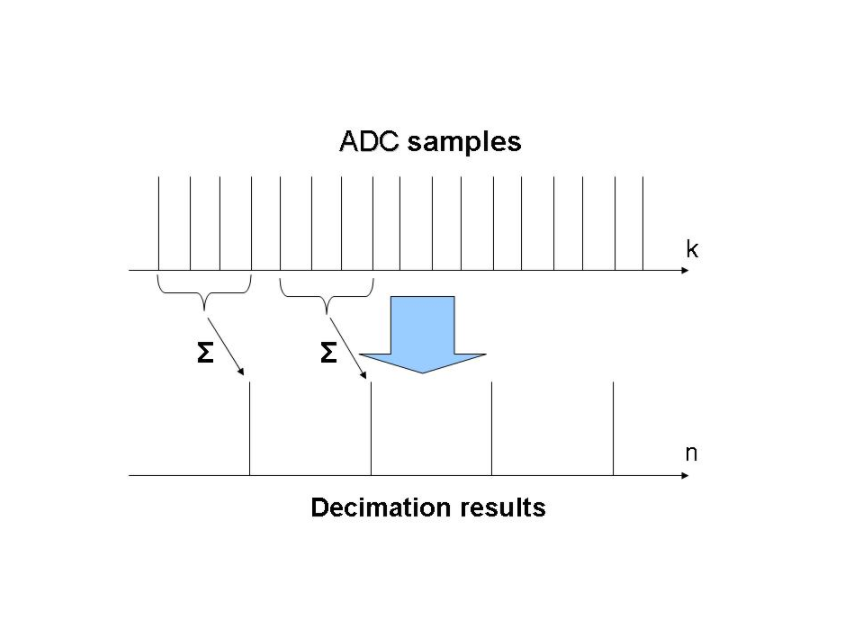
An important factor in the development of digital antenna arrays for radars and Massive MIMO is the need to reduce the cost per channel. Combining the decimation process not only with an anti-aliasing filter, but also with the digital frequency shifting and I/Q-demodulation as well can help to bring down this cost.

In the simpler case of decimation of OFDM signals by an integer factor M, the algorithm^[5] may be used:

[math]\displaystyle{ y[n] = \sum_{k=0}^{M-1} x[nM+k]\ \mathrm e^{-\mathrm i 2\pi f kT}, n=0,1,.., N }[/math],

where [math]\displaystyle{ T }[/math] is interval between samples of signal and [math]\displaystyle{ f }[/math] is the central carrier frequency of the OFDM signal.

For example, setting [math]\displaystyle{ 2\pi f kT = k\pi/2 }[/math] yields the sequence [math]\displaystyle{ e^{-i 2\pi f kT} = 1, e^{-i \pi/2}, e^{-i \pi},... }[/math] and therefore^[5]

[math]\displaystyle{ \operatorname{Re}(y[n]) = \sum_{k=0}^{M-1}( \operatorname{Re}(x[nM+k]) \cos { k \pi/2 } + \operatorname{Im}(x[nM+k]) \sin { k \pi/2 })\, }[/math],

[math]\displaystyle{ \operatorname{Im}(y[n]) = \sum_{k=0}^{M-1}( \operatorname{Im}(x[nM+k]) \cos { k \pi/2 } - \operatorname{Re}(x[nM+k]) \sin { k \pi/2 })\, }[/math].

This algorithm is only one filter of the full discrete Fourier transform and can be useful to decimate samples in an ADC before digital beamforming in digital antenna arrays.

If [math]\displaystyle{ \operatorname{Im}(x[nM+k])=0 }[/math] then ^[6][7]

[math]\displaystyle{ \operatorname{Re}(y[n]) = \sum_{k=0}^{M-1}(\operatorname{Re}(x[nM+k]) \cos { k \pi/2 })\, }[/math],

[math]\displaystyle{ \operatorname{Im}(y[n]) = \sum_{k=0}^{M-1}( \operatorname{Re}(x[nM+k]) \sin { k \pi/2 })\, }[/math],

or

[math]\displaystyle{ \operatorname{Re}(y[n]) = x[nM]-x[nM+2]+x[nM+4]-..., }[/math],

[math]\displaystyle{ \operatorname{Im}(y[n]) = -x[nM+1]+x[nM+3]-x[nM+5]-... }[/math].

Decimation process of ADC samples of digital video signals. https://handwiki.org/wiki/index.php?curid=1522745

For video signals ([math]\displaystyle{ \operatorname{Im}(x[nM+k])=0 }[/math] and [math]\displaystyle{ \operatorname{Re}(x[nM+k])\gt =0 }[/math])

[math]\displaystyle{ y[n] = \sum_{k=0}^{M-1} x[nM+k]\ }[/math].^[8]

If more effective anti-aliasing filtering is required then this method may be modified to produce:

[math]\displaystyle{ y[n] = \sum_{k=0}^{M-1} x[nM+k]h[k]\ \mathrm e^{-\mathrm i 2\pi f kT}, n=0,1,.., N }[/math].

An example of such decimation by [math]\displaystyle{ 2\pi f kT = k\pi/2 }[/math] can be implemented by the formulas:

[math]\displaystyle{ \operatorname{Re}(y[n]) = -6[nM+1]+32x[nM+3]-52x[nM+5]+32x[nM+7]-6x[nM+9], }[/math]

[math]\displaystyle{ \operatorname{Im}(y[n]) = x[nM]-17x[nM+2]+46x[nM+4]-46x[nM+6]+17x[nM+8]-x[nM+10]. }[/math]

A similar combination of filters can be used for decimation using fractional factors.

References

- Strang, Gilbert; Nguyen, Truong (1996-10-01). Wavelets and Filter Banks (2 ed.). Wellesley,MA: Wellesley-Cambridge Press. pp. 100–101. ISBN 0961408871. https://books.google.com/books?id=Z76N_Ab5pp8C&pg=PA101&lpg=PA101&dq=noble+identities+strang&source=bl&ots=qUVRdm_Bh1&sig=j6JbIy66PbqFVdrhigCHnjerNiI&hl=en&sa=X&ei=XKmtUs_FEKbD2AWinIHACQ&ved=0CC8Q6AEwAA#v=onepage&q=noble%20identities%20strang&f=false.
- Realizable low-pass filters have a "skirt", where the response diminishes from near one to near zero. So in practice the cutoff frequency is placed far enough below the theoretical cutoff that the filter's skirt is contained below the theoretical cutoff.
- Some programs (such as MATLAB) that design filters with real-valued coefficients use the Nyquist frequency ([math]\displaystyle{ \tfrac }[/math]) as the normalization constant. That results in a Nyquist frequency of 1 and a periodicity of 2.
- Milić, Ljiljana (2009). Multirate Filtering for Digital Signal Processing. New York: Hershey. p. 192. ISBN 978-1-60566-178-0. "Generally, this approach is applicable when the ratio Fy/Fx is a rational, or an irrational number, and is suitable for the sampling rate increase and for the sampling rate decrease."
- Slyusar V. I. Synthesis of algorithms for measurement of range to M sources with the use of additional gating of the ADC readings.// Radioelectronics and Communications Systems. - Vol. 39. - no. 5. - 1996. - P. 36 – 40. [1]
- T. Schilcher. RF applications in digital signal processing//” Digital signal processing”. Proceedings, CERN Accelerator School, Sigtuna, Sweden, May 31-June 9, 2007. - Geneva, Switzerland: CERN (2008). - P. 258. - DOI: 10.5170/CERN-2008-003. [2]
- Sliusar I.I., Slyusar V.I., Voloshko S.V., Smolyar V.G. Next Generation Optical Access based on N-OFDM with decimation.// Third International Scientific-Practical Conference “Problems of Infocommunications. Science and Technology (PIC S&T’2016)”. – Kharkiv. - October 3 –6, 2016. [3]
- Saska Lindfors, Aarno Pärssinen, Kari A. I. Halonen. A 3-V 230-MHz CMOS Decimation Subsampler.// IEEE transactions on circuits and systems— Vol. 52, No. 2, February 2005. – P. 110.