 +1 credit
| Version | Summary | Created by | Modification | Content Size | Created at | Operation |
|---|---|---|---|---|---|---|
| 1 | Michael Voskoglou | + 2677 word(s) | 2677 | 2020-12-02 05:30:31 | | | |
| 2 | Rui Liu | Meta information modification | 2677 | 2020-12-03 05:27:29 | | | | |
| 3 | Michael Voskoglou | + 5 word(s) | 2682 | 2020-12-03 20:14:06 | | |
Video Upload Options
The theory of Markov chains is a smart combination of Linear Algebra and Probability theory offering ideal conditions for modelling situations depending on random variables. Markov chains have found important applications to many sectors of the human activity. In this work a finite Markov chain is introduced representing mathematically the teaching process which is based on the ideas of constructivism for learning. Interesting conclusions are derived and a measure is obtained for the teaching effectiveness. An example on teaching the derivative to fresher university students is also presented illustrating our results.
1. Introduction
Constructivism is a philosophical framework for learning based on Piaget’s theory and formally introduced by von Clasersfeld during the 1970’s. Constructivism argues that knowledge is not passively received from the environment, but is actively constructed by the learner through a process of adaptation based on and constantly modified by the learner’s experience of the world [1]. The application of the ideas of constructivism in the teaching process has become very popular during the last decades, especially in school education. The steps of a typical framework for teaching which is based on those ideas are the following:
-
Orientation (S1): This is the starting step which connects the past with the present learning experiences and focuses student thinking on the learning outcomes of the current activities.
-
Exploration (S2): In this step students explore their environment to create a common base of experiences by identifying and developing concepts, processes and skills.
-
Formalization (S3): Here students explain and verbalize the concepts that have been explored and the instructor has the opportunity to introduce formal terms, definitions and explanations for the new concepts and processes and demonstrate new skills.
-
Assimilation (S4): In that step students develop a deeper and broader conceptual understanding and obtain more information about areas of interest by practicing on their new skills and behaviors.
-
Assessment (S5): This is the final step of the teaching process, where learners are encouraged to assess their understanding and abilities and teachers evaluate student skills on the new knowledge.
Depending on the student reactions in the classroom, there are forward or backward transitions between the three intermediate steps (S2, S3 and S4) of this framework during the teaching process, the flow-diagram of which is shown in Figure 1.

Figure 1: The flow-diagram of the teaching process
In this article a Markov chain is introduced on the steps of the teaching process and through it interesting conclusions are derived for the teaching effectiveness.
2. Markov Chains
Roughly speaking a Markov chain (MC) is a stochastic process that moves in a sequence of steps (phases) through a set of states and has a one-step memory. In other words, the probability of entering a certain state in a certain step depends on the state occupied in the previous step and not in earlier steps. This is known as the Markov property. However, for being able to model as many real life situations as possible by using MCs, one could accept in practice that the probability of entering a certain state in a certain step, although it may not be completely independent of previous steps, it mainly depends on the state occupied in the previous step [2].
The basic concepts of MCs were introduced by Andrey Markov (Figure 2) in 1907 on coding literal texts.
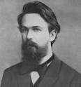
Figure 2: A. Markov (1856-1922).
Since then the MC theory was developed by a number of leading mathematicians, such as A. Kolmogorov, W. Feller, etc. However, only from the 1960’s the importance of this theory to the natural, social and applied sciences has been recognized [3][4][5][6][7][8].
2.1 Finite Markov Chains
When the set of states of a MC is a finite set, then we speak about a finite MC. For general facts on finite MCs we refer to Chapter 2 of the book [9].
Let us consider a finite MC with n states, say S1, S2, …, Sn, where n is a nonnegative integer, n 2. Denote by pij the transition probability from state Si to state Sj , i, j = 1, 2,…, n ; then the matrix A= [pij] is called the transition matrix of the MC. Since the transition from a state to any other state (including its self) is the certain event, we have that
pi1 + pi2 + . + pin , i = 1, 2,., n (1)
The row-matrix Pk = [p1(k) p2(k)… pn(k)], known as the probability vector of the MC, gives the probabilities pi(k) for the MC to be in state i at step k , for i = 1, 2,…., n and k = 0, 1, 2,…. Obviously we have again that
Using conditional probabilities on can show ([9], Chapter 2, Proposition 1) that for all nonnegative integers k is
Pk+1= Pk A (3).
Then, a straightforward induction on k gives that
Pk =Po Ak (4) .
Equations (3) and (4) enable one to make short run forecasts for the evolution of the various situations that can be represented by a finite MC. In practical applications we usually distinguish between two types of finite MCs, the absorbing MCs (AMCs) and the ergodic MCs (EMCs).
2.2. Absorbing Markov Chains
A state of a MC is called absorbing if, once entered, it cannot be left. Further a MC is said to be an AMC if it has at least one absorbing state and if from every state it is possible to reach an absorbing state, not necessarily in one step.
Working with an AMC with k absorbing states, 1 k < n, one brings its transition matrix A to its canonical (or standard) form A* by listing the absorbing states first and then makes a partition of A* to sub-matrices as follows
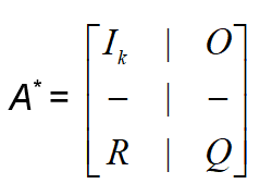
In the above partition of A*, Ik denotes the unitary k X k matrix, O is a zero matrix, R is the (n – k) X k transition matrix from the non-absorbing to the absorbing states and Q is the (n – k) X (n – k) transition matrix between the non-absorbing states.
It can be shown ([10], Section 2) that the square matrix In – k - Q, where In – k denotes the unitary n-k X n-k matrix is always an invertible matrix. The fundamental matrix N of the AMC is defined to be the inverse matrix of In–k – Q. Therefore ([11], Section 2.4).
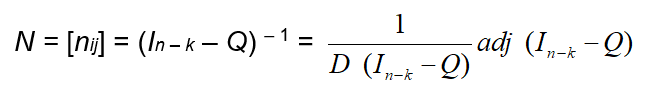
In equation (6) D (In – k – Q) and adj (In–k – Q) denote the determinant and the adjoin of the matrix In – k – Q respectively It is recalled that the adjoin of a matrix M is the matrix of the algebraic complements of the transpose matrix Mt of M, which is obtained by turning the rows of M to columns and vice versa. It is also recalled that the algebraic complement mij΄of an element mij of M is calculated by the equation
mij΄ = (-1)i+jDij (7)
In equation (7) Dij denotes the determinant of the matrix obtained by deleting the i-th row and the j-th column of M.
It is well known ([5], Chapter 3) that the element nij of the fundamental matrix N gives the mean number of times in state Si before the absorption, when the starting state of the AMC is Sj , where Si and Sj are non-absorbing states.
2.3. Ergodic Markov Chains
A MC is said to be an EMC, if it is possible to go between any two states, not necessarily in one step. It is well known ([5], Theorem 5.1.1) that, as the number of its steps tends to infinity (long run), an EMC tends to an equilibrium situation, in which the probability vector Pk takes a constant price P = [p1 p2 …. pn], called the limiting probability vector of the EMC. Therefore, as a direct consequence of equation (3), the equilibrium situation is characterized by the equation
P = PA, with p1+ p2+ ….+ pn = 1 (8)
The entries of P express the probabilities of the EMC to be in each of its states in the long run, or in other words the importance (gravity) of each state of the EMC.
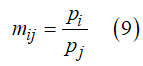
Let us now demote with mij the mean number of times in state Si between two successive occurrences of the state Sj, i, j = 1, 2, …., n. It is well known ([5], Theorem 6.2.3) then that
3. A Markov Chain Model for the Teaching Process
3.1. The Model
Here we introduce a finite MC having as states Si, i = 1, 2,…, 5, the corresponding steps of the teaching framework described in our Introduction. From the flow-diagram of Figure 1 it becomes evident that this chain is an AMC with S1 being its starting state and S5 being its unique absorbing state. The minimum number of steps before the absorption is 4 and this happens when we have no backward transitions between the three middle states S2, S3 and S4 of the chain. Denote by pij the transition probability of the MC from state Si to state Sj, for i, j =1, 2,…,5. Then the transition matrix A of the chain and its canonical form A* are the following:
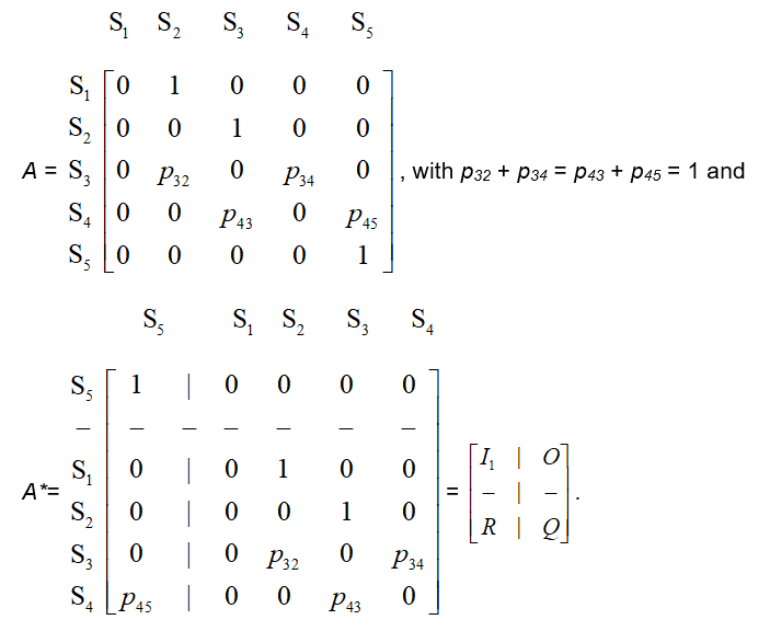
Denote by I4 the 4X4 unitary matrix. Then the fundamental matrix of the AMC is
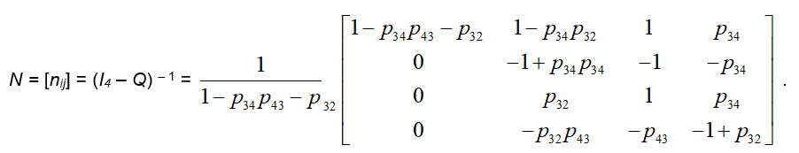
Therefore, since S1 is the starting state of the above AMC, it becomes evident that the mean number of steps before the absorption is given by the sum
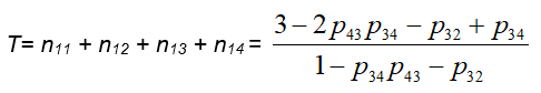
It becomes evident too that the bigger is T, the more are the student difficulties during the teaching process. Another factor of the student difficulties is the total time spent for the completion of the teaching process. However, the time is usually fixed in a formal teaching procedure in the classroom, which means that in this case T is the unique measure of the student difficulties.
3.2. A Classroom Application
The present application took place at the Graduate Technological Educational Institute of Western Greece for teaching the concept of the derivative to a group of fresher students of engineering. The instructor used the teaching framework that has been described in our Introduction as follows:
Orientation: The student attention was turned to the fact that the definition of the tangent of a circle as a straight line having a unique common point with its circumference does not hold for other curves (e.g. for the parabola). Therefore, there is a need to search for a definition of the tangent covering all cases and in particular of the tangent at a point of the graph of a given function.
Exploration: The discussion in the class led to the conclusion that the tangent at a point A of the graph of a given function y=f(x) can be considered as the limit position of the secant line of the graph through the points Α(a, f(a)) and Β(b, f(b)), when the point Β is moving approaching to Α either from the left, or from the right (Figure 3). But the slope of the secant line AB is equal to 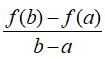
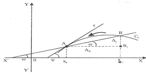
Figure 3: Tangent at a point of the graph of a given function
Formalization: Based on what it has been discussed at the step of exploration, the instructor presented the formal definition of the derivative number f΄(a) at a point Α(a, f(a)) of a given function y=f(x) as the limit (if there exists) of 
Assimilation: Here the fact that the derivative y΄ = f΄(x) expresses the rate of change of the function y=f(x) with respect to x was emphasized and its physical meaning was also presented connected to the speed and the acceleration at a moment of time of a moving object under the action of a steady force. The fundamental properties of the derivatives followed (sum, product, composite function, etc.) as well as a list of formulas calculating the derivatives of the basic functions and applications of them.
It has been observed that the student reactions during the teaching process led to 2 transitions of the discussion from state S3 (formalization) back to state S2 (exploration). Therefore, since from state S2 the chain moves always to S3 (Figure 1), we had 3 in total transitions from S2 to S3. The instructor also observed 3 transitions from S4 (assimilation) back to S3. Therefore, since from state S3 the chain moves always to state S4 (Figure 1), we had 4 in total transitions from S3 to S4. In other words we had 3+3 = 6 in total “arrivals” to S3, 2 “departures” from S3 to S2 and 4 “departures” from S3 to S4. Therefore p32 = 2/6 and p34 = 4/6. In the same way one finds that p43 = 3/4 and p45 = 1/4. Replacing the above values of the transition probabilities to equation (10) one finds that the mean number T of steps before the absorption of the MC is equal to 14. Consequently, since the minimum number of steps before the absorption is 4, the students faced significant difficulties during the teaching process. This means that the instructor should find ways to improve his teaching procedure of the same subject in future.
3.3. An Important Remark
In certain cases it is possible to develop either an AMC or an EMC model for representing the same situation. In case of the teaching process, for example, the flow diagram of Figure 1 could be revised by assuming that, when the teaching process of a subject matter is integrated, then a new process starts by the instructor for teaching the next subject of the course. That means that the teaching process is transferred back from step S5 to S1 to be repeated from the beginning again. The revised flow diagram of the teaching process, therefore, takes the form of Figure 4.
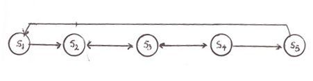
Figure 4: Revised flow diagram of the teaching process
In this case the resulting MC on the steps of the teaching process is obviously an EMC. Since S1 is the starting state of the EMC it becomes evident that the sum m=m15+m25+m35+m45 calculates the mean number of steps of the EMC between two successive occurrences of the state S5. Therefore, the mean number of steps for the completion of the teaching process will be m+1, since it includes also the step S5. With the help of equation (9) one finds that
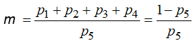
The value of the limiting probability p5 is calculated with the help of the matrix equation (8). In this equation the transition matrix of the EMC differs from the corresponding matrix A of the AMC of section 3.1only with respect to the last row, where 1 is transferred from the fifth to the first column and its other entries are 0. Performing the necessary calculations, equation (8) leads to a linear system of five equations with respect to the pi’s, i = 1, 2, 3, 4, 5. Adding by members the first four of those equations one finds the fifth one. Thus, replacing the fifth equation with the equation p1+p2+p3+p4+p5 = 1 and solving the resulting 5X5 linear system one finds the required value of p5 and with the help of equation (11) calculates m (for more details see [9], pp. 62-63). It becomes evident that, the greater is the value of m the more the student difficulties during the teaching process. Concerning the classroom application of section 3.2 , after performing all the necessary calculations one finds that m+1 = T.
4. Conclusion
In the paper at hands a mathematical representation of the teaching process based on the principles of constructivism for learning was developed with the help of the theory of MCs. This representation enables the instructor to evaluate the student difficulties during the teaching process, which is very useful for reorganizing the plans for teaching the same subject in future. Although the theoretical development of the MC model is quite laborious, its final application in practice is too easy and straightforward. It requires only to count the backward movements among the three middle steps S2, S3 and S4 of the teaching process. The theory of MCs can be used for several other applications in Education (e.g. see Chapter 3 of [9]) and this is one of the main targets of our future research.
References
- Taber, K.S. Chapter 2: Constructivism as educational theory: Contingency in learning, and optimally guided instruction. in Educational Theory; J. Hassaskhah, Eds.; Nova Science Publishers: NY, USA, 2011; pp. 39-61.
- Kemeny, J.G., Schleifer, A.J. & Snell, J.L, Finite Mathematics with Business Applications, Prentice Hall, London, 1962.
- Suppes, P.; Atkinson, R. C.. Markov Learning Models for Multiperson Interactions; Stanford University Press: Stanford-California, USA, 1960; pp. 1-.
- Bartholomew, R.C.. Stochastic Models for Social Processes; J. Wiley and Sons: London, UK, 1973; pp. 1-.
- Kemeny, J.; Snell, J. l.. Finite Markov Chains; Springer-Verlag: New York, USA, 1976; pp. 1-.
- Domingos, P.; Lowd, D.. Markov Logic: An Interface Layer for Artificial Intelligence; Morgan & Claypool Publishers: Williston, VT, USA, 2009; pp. 1-.
- Zucchini, I.L.; MacDonald, I.L.; Langrock, R.. Hidden Markov Models for Time Series; CRC Press: NY, USA, 2009; pp. 1-.
- Davis, M.H.A.. Markov Models and Optimization ; Create Space Independent Publishing Platform: Columbia, SC., USA, 2017; pp. 1-.
- Voskoglou, M.Gr.. Finite Markov Chain and Fuzzy Logic Assessment Models: Emerging Research and Opportunities ; Create Space Independent Publishing Platform (Amazon): Columbia, SC, USA, 2017; pp. 1-.
- M. G. Voskoglou; S. Perdikaris; A Markov chain model in problem solving. International Journal of Mathematical Education in Science and Technology 1991, 22, 909-914, 10.1080/0020739910220607.
- Morris, A.O.. An Introduction to Linear Algebra, ; Van Nostrand Beinhold Company Ltd.: Berkshire, England, 1978; pp. 1-.

