 +1 credit
| Version | Summary | Created by | Modification | Content Size | Created at | Operation |
|---|---|---|---|---|---|---|
| 1 | G.-Fivos Sargentis | + 1388 word(s) | 1388 | 2020-11-17 13:50:15 | | | |
| 2 | G.-Fivos Sargentis | Meta information modification | 1388 | 2020-11-23 18:13:31 | | | | |
| 3 | G.-Fivos Sargentis | Meta information modification | 1388 | 2020-11-23 18:14:48 | | | | |
| 4 | Catherine Yang | Meta information modification | 1388 | 2020-11-24 02:50:25 | | |
Video Upload Options
Stochastic calculus is used for the objective evaluation of the variability present in aesthetic attributes of paintings and landscapes.
1. Introduction
The aesthetic evaluation of art paintings typically involves the physical procedure of visual examination of an image. This approach is considered highly subjective and celebrated as such, with its outcomes being the subject of philosophy of art, in particular of the philosophical branch known as aesthetics. In an attempt to conceive an alternative, objective procedure for aesthetic analysis, a plethora of studies have employed mathematical algorithms and quantitative metrics for image evaluation and classification. In the realm of quantitative art studies, stochastic analysis offers an advantageous and innovative framework for examining art paintings under the prism of randomness.
In particular, the mathematical field of Stochastics has been introduced as an alternative to deterministic approaches and is used to model the so-called random, i.e., complex, unexplained or unpredictable, fluctuations observed in (but not limited to) non-linear geophysical processes [1] [2] [3]. Stochastics helps develop a unified perception for natural phenomena and expel dichotomies like random vs. deterministic. Under the viewpoint of stochastics, there is no such thing as a virus of randomness that infects some phenomena to make them random, leaving other phenomena unaffected. Rather it seems that both randomness and predictability coexist and are intrinsic to natural systems, which can be deterministic and random at the same time, depending on the prediction horizon and the time scale [4]. On this basis, the uncertainty in art, in line with other natural processes, could be considered both aleatory and epistemic (since, in principle, we do not know perfectly well the underlying causal mechanisms). By applying the methods of stochastics, we can quantify this uncertainty treating the unpredictable fluctuations of art works as realizations of complex stochastic processes.
A physical process is characterized as complex when it is difficult to analyze or explain in a completely predictive way. Likewise, constructions by artists (e.g., paintings, music, literature, etc.) are also expected to be of high complexity since they are produced by numerous human (e.g., logic, intuition, emotions, etc.) and non-human (e.g., quality of paints, paper, tools, etc.) processes interacting with each other in a complex manner. Art paintings, being the result of various processes interacting with each other at multiple scales, are thus likely to resemble a stochastic process of increased uncertainty and variability. Such a process deviates from a purely White-Noise behavior, as its aesthetic attributes are likely to appear in clusters by a highly non-predictive manner.
Even though beauty is difficult or even impossible to quantify, nevertheless stochastic analysis may offer new insights into aesthetical issues and a basis for their objective evaluation. The stochastic analysis of the examined artworks is performed using the 2D-climacogram (2D-C), a stochastic tool evaluating the degree of variability vs spatial scale.
2. Data, Model, Applications and Influences
2.1. Stochastic Analysis in 2D
Α stochastic computational tool called 2D-C [5][6] is used to analyze images of art paintings quantifying the variability of the brightness vs scale in a specific image and in a group of images as well. Here, we refer to spatial (not time) scale, defined as the ratio of the area of k × k adjacent cells (i.e., scale k) that are averaged to form the (scaled) spatial field, over the spatial resolution of the original field (i.e., at scale 1). The term climacogram [7][8] comes from the greek word climax (meaning scale). It is defined as the (plot of) variance of the averaged process (assuming stationary) versus averaging scale k, and is denoted as γ(k). The climacogram is useful for detecting the long-term change (or else dependence, persistence, clustering) of a process, which emerges particularly in complex systems as opposed to white-noise (absence of dependence) of even Markov (i.e., short-term persistence) behaviour [9].
In order to obtain a quantitative characterization of the artwork, its image is digitized in 2D and each pixel is assigned a grayscale color intensity (white = 1, black = 0). Assuming that our sample is an area nΔ × nΔ, where n is the number of intervals (e.g., pixels) along each spatial direction and Δ is the discretization unit determined by the image resolution, (e.g., pixel length), the empirical classical estimator of the climacogram for a 2D process can be expressed as:
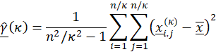 |
(1) |
where the ‘^’ over γ denotes estimation, is the the dimensionless spatial scale, 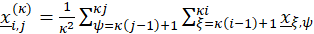

An important property of stochastic processes is the Hurst–Kolmogorov (HK) dynamics (usually known in hydrometeorological processes as Long-Term Persistence, or LTP), which can be summarized by the Hurst parameter as estimated in large scales. This parameter is estimated by minimizing the fitting error of the logarithmic slope of the tail (i.e., the last 50 scales in the presented applications) of the observed (from data through Eqn. 1) and the modelled (Eqn. 2) climacogram. The isotropic HK process with an arbitrary marginal distribution (e.g., for the Gaussian one, this results in the well-known fractional-Gaussian-noise, as described by Mandelbrot and van Ness [10], i.e., the power-law decay of variance as a function of scale, is defined for a 1D or 2D process as:
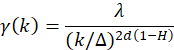 |
(2) |
where is the variance at scale k = κΔ, d is the dimension of the process/field (i.e., for a 1D process d = 1, for a 2D field d = 2, etc.), and H is the Hurst parameter (0 < H < 1). For 0 < H < 0.5 the HK process exhibits an anti-persistent behavior, H = 0.5 corresponds to the white noise process, and for 0.5 < H < 1 the process exhibits LTP (clustering). In the case of clustering behavior, due to the non-uniform heterogeneity of the brightness of the painting, the high variability in brightness persists even in large scales. This clustering effect may substantially increase the diversity between the brightness in each pixel of the image, a phenomenon also observed in hydrometeorological processes (such as temperature, precipitation, wind etc.), natural landscapes and music [11].
The algorithm that generates the climacogram in 2D was developed in MATLAB for rectangular images [12]. In particular, for the current analysis, the images are cropped to 400 × 400 pixels, 14.11 cm × 14.11 cm, in 72 dpi (dots per inc).
2.2. Illustration of Stochastic Analysis in 2D
The pixels analyzed are actually represented by numbers based on their grayscale color intensity (white = 1, black = 0). Figure 1 presents three images for benchmark image analysis: (a) white noise; (b) image with clustering; and (c) an art painting. Figure 2 presents the steps of our analysis, and shows how grouped pixels at scales k = 2, 4, 8, 16, 20, 25, 40, 50, 80, 100 and 200, are used to calculate the climacogram. Figures 1 and 2 present an example of how we can estimate the climacograms and standardized climacograms from the data sets in Figure 2. The standardized climacogram, which is the basic tool of the 2D-C evaluation process, is defined as the ratio , and it is also a function of scale k but without having any effect from the marginal variance of the process.
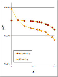
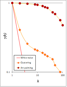
The presence of clustering is reflected in the climacogram, which shows a marked difference compared to independent pixels as in white noise processes (Figure 2). Specifically, the variance of the clustered images is notably higher than that of white noise at all scales, indicating a greater degree of variability and uncertainty of the process. Likewise, comparing the clustered image and the art painting, the latter has the most pronounced clustering behavior and a higher degree of variability.
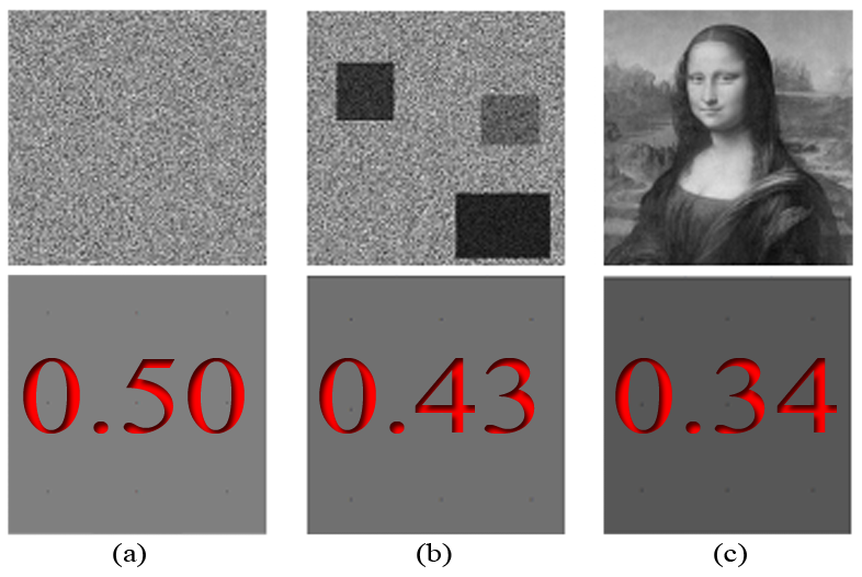
Figure 1. Benchmark of image analysis; (a) White noise; (b) Image with clustering; (c) Art painting; the lower row depicts the average brightness in the upper one.
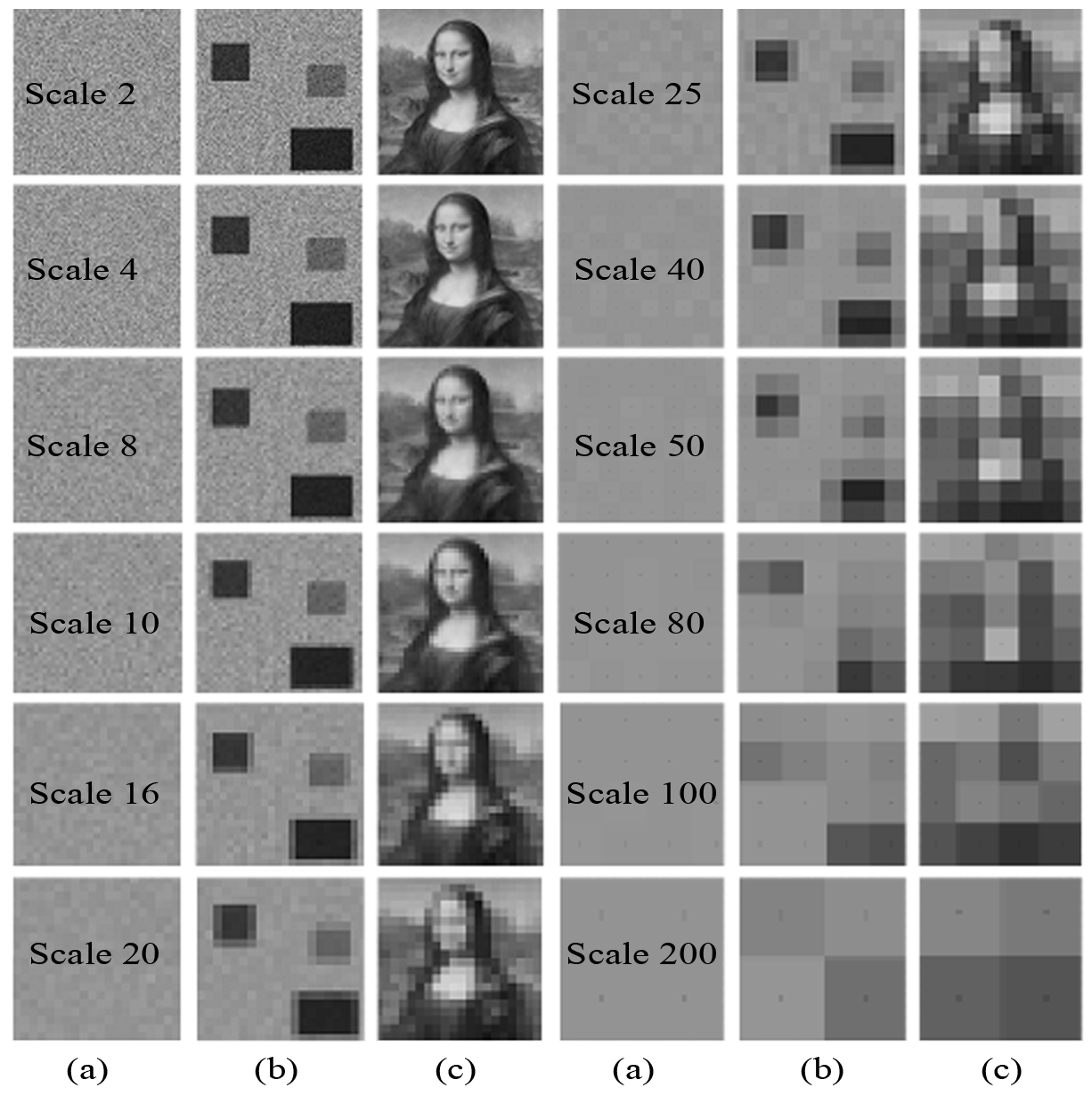
Figure 2. Example of stochastic analysis of 2D picture; steps. Grouped pixels at different scales used to calculate the climacogram; (a) White noise; (b) Image with clustering; (c) Art painting.
 |
 |
| (a) | (b) |
Figure 3. (a) Climacograms of the benchmark images; (b) Standardized climacograms of the benchmark images.
The results of stochastic analysis are presented in papers: [5][6][13][14][15][16].
References
- Koutsoyiannis, D.: HESS Opinions "A random walk on water", Hydrol. Earth Syst. Sci., 14, 585–601, https://doi.org/10.5194/hess-14-585-2010, 2010.
- Dimitriadis, P., Hurst-Kolmogorov dynamics in hydrometeorological processes and in the microscale of turbulence, PhD thesis, Department of Water Resources and Environmental Engineering – National Technical University of Athens, 2017.
- D. Koutsoyiannis, Stochastics of Hydroclimatic Extremes - A Cool Look at Risk, 330 pages, Edition 0, National Technical University of Athens, Athens, 2020.
- Panayiotis Dimitriadis; Aristoteles Tegos; Athanasios Oikonomou; Vassiliki Pagana; Antonios Koukouvinos; Nikos Mamassis; Demetris Koutsoyiannis; Andreas Efstratiadis; Comparative evaluation of 1D and quasi-2D hydraulic models based on benchmark and real-world applications for uncertainty assessment in flood mapping. Journal of Hydrology 2016, 534, 478-492, 10.1016/j.jhydrol.2016.01.020.
- G.-Fivos Sargentis; Panayiotis Dimitriadis; Romanos Ioannidis; Theano Iliopoulou; Demetris Koutsoyiannis; Stochastic Evaluation of Landscapes Transformed by Renewable Energy Installations and Civil Works. Energies 2019, 12, 2817, 10.3390/en12142817.
- G.-Fivos Sargentis; Panayiotis Dimitriadis; Demetris Koutsoyiannis; Aesthetical Issues of Leonardo Da Vinci’s and Pablo Picasso’s Paintings with Stochastic Evaluation. Heritage 2020, 3, 283-305, 10.3390/heritage3020017.
- Koutsoyiannis, D. (2013), Encolpion of stochastics: Fundamentals of stochastic processes, 12 pages, Department of Water Resources and Environmental Engineering – National Technical University of Athens, Athens
- Koutsoyiannis, D. (2013b), Climacogram-based pseudospectrum: a simple tool to assess scaling properties, European Geosciences Union General Assembly 2013, Geophysical Research Abstracts, Vol. 15, 700 Vienna, EGU2013-4209, European Geosciences Union.
- Panayiotis Dimitriadis; Demetris Koutsoyiannis; Climacogram versus autocovariance and power spectrum in stochastic modelling for Markovian and Hurst–Kolmogorov processes. Stochastic Environmental Research and Risk Assessment 2015, 29, 1649-1669, 10.1007/s00477-015-1023-7.
- Benoit B. Mandelbrot; John W. Van Ness; Fractional Brownian Motions, Fractional Noises and Applications. SIAM Review 1968, 10, 422-437, 10.1137/1010093.
- Sargentis, G.-F.; Dimitriadis, P.; Iliopoulou, T.; Ioannidis, R.; Koutsoyiannis, D., Stochastic investigation of the Hurst-Kolmogorov behaviour in arts, European Geosciences Union General Assembly 2018, Geophysical Research Abstracts, Vol. 20, Vienna, EGU2018-17082, European Geosciences Union, 2018.
- Panayiotis Dimitriadis; Katerina Tzouka; Demetris Koutsoyiannis; Hristos Tyralis; Anna Kalamioti; Eleutherios Lerias; Panagiotis Voudouris; Stochastic investigation of long-term persistence in two-dimensional images of rocks. Spatial Statistics 2019, 29, 177-191, 10.1016/j.spasta.2018.11.002.
- Sargentis, G.-F.; Ioannidis, R.; Meletopoulos, I. T.; Dimitriadis, P.; Koutsoyiannis, D., Aesthetical issues with stochastic evaluation, European Geosciences Union General Assembly 2020, Geophysical Research Abstracts, Vol. 22, Online, EGU2020- 19832, https://doi.org/10.5194/egusphere-egu2020-19832, European Geosciences Union, 2020.
- Manta, E.; Ioannidis, R.; Sargentis, G.-F.; Efstratiadis, A., Aesthetic evaluation of wind turbines in stochastic setting: Case study of Tinos island, Greece, Aesthetic evaluation of wind turbines in stochastic setting: Case study of Tinos island, Greece, European Geosciences Union General Assembly 2020, Geophysical Research Abstracts, Vol. 22, Online, EGU2020- 5484, https://doi.org/10.5194/egusphere-egu2020-5484, European Geosciences Union, 2020.
- Ioannidis, R., Dimitriadis, P.; Meletopoulos, I. T.; Sargentis, G.-F.; Koutsoyiannis, D., Investigating the spatial characteristics of GIS visibility analyses and their correlation to visual impact perception with stochastic tools, European Geosciences Union General Assembly 2020, Geophysical Research Abstracts, Vol. 22, Online, EGU2020- 18212, https://doi.org/10.5194/egusphere-egu2020-18212, European Geosciences Union, 2020.
- Ioannidis, R.; Dimitriadis, P.; Sargentis, G.-F.; Frangedaki, E.; Iliopoulou, T.; Koutsoyiannis, D., Stochastic similarities between hydrometeorogical and art processes for optimizing architecture and landscape aesthetic parameters, European Geosciences Union General Assembly 2019, Geophysical Research Abstracts, Vol. 21, Vienna, EGU2019-11403, European Geosciences Union, 2019.

