Applications of E-Nose in Tea Quality Evaluation

Version	Summary	Created by	Modification	Content Size	Created at	Operation
1		Ho-Hsien Chen	--	3521	2022-09-27 17:59:59	\|
2	Reference format revised.	Lindsay Dong	Meta information modification	3521	2022-09-28 04:07:01	\|

This entry is adapted from the peer-reviewed paper 10.3390/agriculture12091359

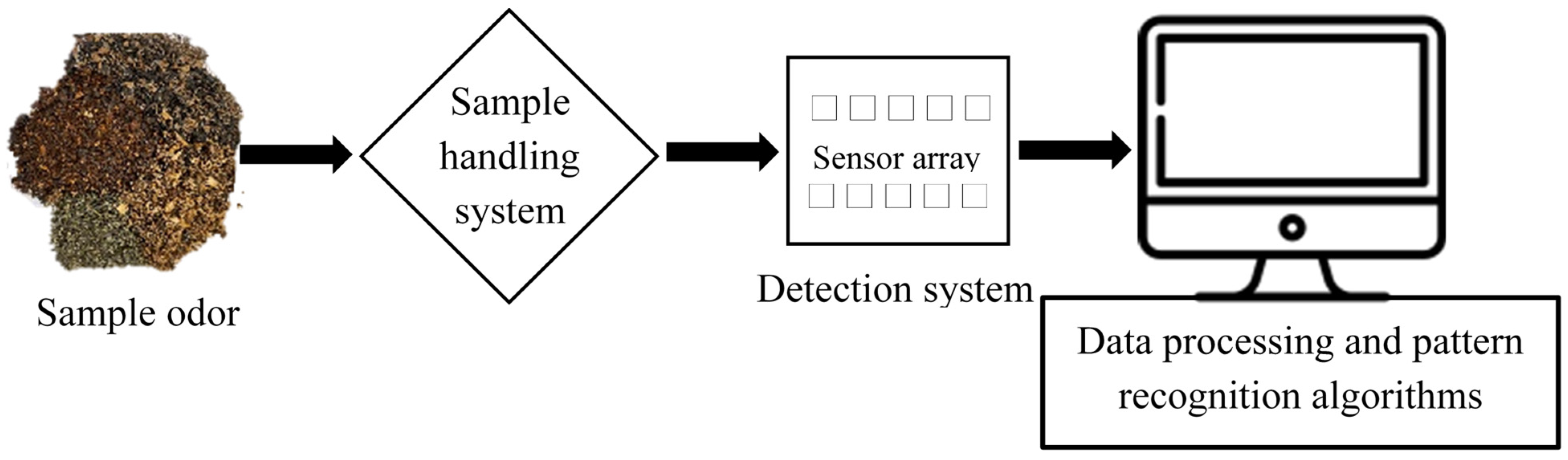
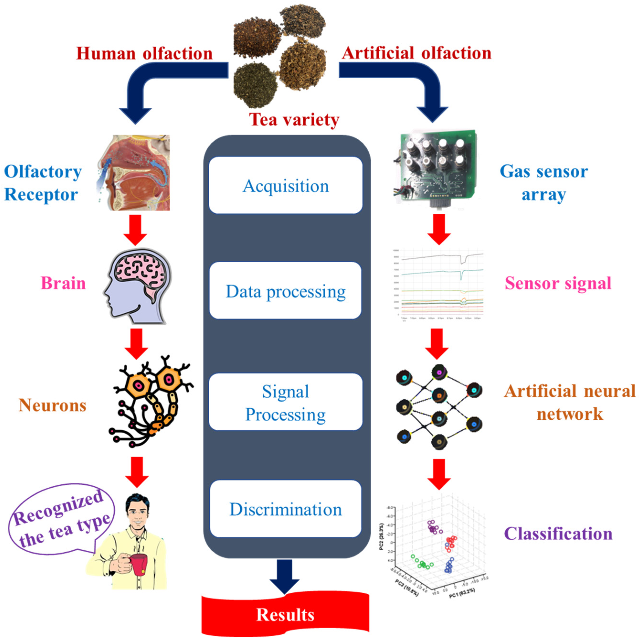
The advancement in sensor technology has replaced the human olfaction system with an artificial olfaction system, i.e., electronic noses (E-noses) for quality control of teas to differentiate the distinct aromas. An E-nose system’s sensor array consists of some non-specific sensors, and an odor stimulus generates a fingerprint from this array. Fingerprints or patterns from known odors are used to train a pattern recognition model such that unknown odors can be classified and identified subsequently. Recently, the E-nose has been regarded as a powerful tool for tea quality monitoring. For instance, wide applications in tea research include tea classification, tea fermentation methods, tea components, tea grade quality, and tea storage.

aroma electronic nose gas sensors intelligent pattern recognition tea quality

1. Introduction

Usually, human sensory analysis is used to assess the quality of tea based on sensory descriptors, namely morphological characteristics, tastes, aromas, texture, and colors ^[1]^[2]. The analysis requires professional panel evaluators to have their own perceptions about various tea sensory attributes, which is difficult for consumers to understand. Besides, the main problems of sensory analysis are the need for a large group of educated and trained people (not always feasible) ^[3], long and constant training, harmonization of vocabulary, and special technical conditions (such as room and lighting). In recent years, numerous analytical techniques have been proposed for assessing tea quality: for example, ultraperformance liquid chromatography (UPLC), high-performance liquid chromatography (HPLC), gas chromatography-mass spectrometry (GC-MS), capillary electrophoresis (CE), and plasma atomic emission spectrometry ^[1]^[2]. These methods, however, have disadvantages in that they impose high operation costs, require highly skilled analysts and time-consuming techniques, and cannot be applied for real-time monitoring of tea quality ^[2]^[4]^[5]. Therefore, the higher expectations for quality control of products have increased the requirements for rapid, reliable, and cost-effective analysis.

With the rapid advancement of multi-sensor and electronic technologies, accurate results in fast food analysis have become possible. Electronic eye (E-eye), electronic nose (E-nose), and electronic tongue (E-tongue) systems are composed of color, gas, and liquid sensors that resemble human vision, olfactory, and gustatory systems. The sample detection is fast, with no requirement for sample pretreatment ^[6]. An E-nose system has been developed to identify and distinguish different odors ^[7]. An E-nose system’s sensor array consists of some non-specific sensors, and an odor stimulus generates a fingerprint from this array. Fingerprints or patterns from known odors are used to train a pattern recognition model such that unknown odors can be classified and identified subsequently ^[3]. Recently, the E-nose has been regarded as a powerful tool for tea quality monitoring. For instance, wide applications in tea research include tea classification, tea fermentation methods, tea components, tea grade quality, and tea storage ^[3]^[4].

2. E-Nose Instrumentation

The E-nose device is designed in such a manner as to identify and distinguish between a variety of complex odors. This non-destructive device is composed of sensor arrays that react to the vapors and gases the sample generates. Typically, the sensor array comprises non-specific sensors that have been sensitized to various chemical substances; thus, each element measures a distinct property of the chemical perceived ^[8]. When the odors or volatile molecules react with the sensor array, subsequent changes in the electrical properties, mainly conductivity, occur. As a consequence, pattern recognition algorithms are used to characterize those detected changes to perform classification or discrimination of samples ^[9]. As represented in Figure 1, the E-nose device consists of three main parts: (1) sample handling system, (2) detection system, and (3) data processing system and pattern recognition algorithms. A comparison of the basic analogies between human olfaction (biological olfaction) and an E-nose (artificial olfaction) is represented in Figure 2.

/media/item_content/202209/6333aa6672929agriculture-12-01359-g001.png

Figure 1. A schematic representation of the E-nose system.

/media/item_content/202209/6333aa756da83agriculture-12-01359-g002.png

Figure 2. Illustration representing the analogy between human olfaction and artificial olfaction.

3. Pattern Recognition Algorithms for E-Nose

Pattern recognition constitutes an important part in the development of an E-nose instrument capable of detection, identification, and quantification of different complex volatile compounds. These are typically classified as statistical and intelligent pattern recognition methods ^[10]. The most widely applied pattern recognition techniques in E-nose applications include linear discriminant analysis (LDA) and discriminant function analysis (DFA), principal component analysis (PCA), multinomial logistic regression (MultiLR), partial least squares discriminant analysis (PLS-DA), partial least squares regression (PLSR), hierarchical cluster analysis (HCA), K-nearest neighbor (KNN), artificial neural network (ANN), convolutional neural network (CNN), decision trees (DT), random forest (RF), and support vector machine (SVM) ^[10]^[11]. PCA and HCA are unsupervised learning algorithms, while LDA and DFA, MultiLR, PLS-DA, PLSR, KNN, ANN, CNN, DT, RF, and SVM are supervised learning algorithms ^[12]. These algorithms can be categorized into statistical or intelligent pattern recognition methods based on linear or nonlinear approaches ^[9]^[10]^[13].

3.1. Statistical Pattern Recognition Methods

3.1.1. Linear Discriminant Analysis (LDA)

LDA, a dimensionality reduction technique, is a widely applied recognition method for E-nose devices. This method identifies a linear combination of features that characterize or distinguish between two or more classes of odors ^[14]. Suppose there are two classes of odors in samples. LDA creates one hyperplane and projects the data in such a way that the separation of classes is maximized. The hyperplane is drawn based on minimizing the distance within the same class and maximizing the distance between the classes ^[15]. The purpose of LDA is to reduce the original dataset into a lower-dimensional space with high sample discrimination, thus reducing the risk of overfitting and computing costs ^[16]. The requirements of LDA include continuous quantities of the input independent variables for given observations ^[14].

3.1.2. Principal Component Analysis (PCA)

PCA is a statistical method belonging to the factorial analysis group. PCA aims to use a small number of factors to represent the variance in a dataset ^[17]. Using an orthogonal transformation, it converts a set of observations of possibly correlated variables into a set of values of linearly uncorrelated variables. These variables are known as principal components (PCs) ^[14]. Iteratively calculated PCs retain as much variance as possible from the original data, such that PC1 accounts for more data variance than PC2, and PC2 accounts for more data variance than PC3, and so on. Because of this, a few PCs account for the variability in a large number of original data sets. For PCA analysis, only PCs having eigen values greater than 1 are considered significant based on the Kaiser criterion. In contrast, Bartlett’s test of sphericity indicates the suitability of the raw data for performing PCA ^[17].

3.1.3. Multinomial Logistic Regression (MultiLR)

MultiLR is an extension of the logistic (binary) regression model. This method is used when the dependent variable of a study has more than two categorical levels of outcome variable. MultiLR, like binary logistic regression, employs maximum likelihood estimation to determine the probability of categorical membership ^[18]. MultiLR is a classification approach with a discrete random variable set of 1,2,3, …, K, where K is the number of categories. The independent variable is either 0 or 1. Several studies have employed the application of MultiLR to create classification models with good classification results ^[19]. MultiLR has gained much popularity because it does not require assumptions of normality, linearity, and homogeneity of variance of independent variables. Hence, it is a more commonly used method of analysis than discriminant function analysis since it does not require such assumptions ^[20].

3.1.4. Partial Least Squares Discriminant Analysis (PLS-DA)

The PLS algorithm was earlier used for regression analysis and later developed into the PLS-DA classification approach (PLS-DA). PLS-DA has been used in practice for both predictive and descriptive modelling, as well as the selection of discriminative variables ^[21]. PLS-DA is a dimensionality reduction technique that is referred to as a supervised version of PCA. It can be used for feature selection and classification as well. It seeks to find linear transformations that transform data to a lower dimensional space with the least amount of error via optimizing separation between samples of different groups ^[22]. Furthermore, PLS-DA does not require the data to fit a specific distribution, making it more flexible compared to other discriminant methods such as Fisher’s LDA. Several researchers have reported a wide range of applications of PLS-DA modelling in food analysis and metabolomics ^[21].

3.1.5. Partial Least Squares Regression (PLSR)

The PLSR technique combines and generalizes the features of PCA and MLR (multiple linear regression). Its aim is to predict a set of dependent variables from a set of independent variables. This prediction is accomplished by extracting a set of orthogonal factors (known as latent variables) from the predictors having the highest predictive ability. This technique is especially useful when a dependent variable set needs to be predicted from a large independent variable set ^[23]. The PLSR model finds the relationship between two data matrices, X and Y. In addition, it goes beyond the traditional regression by modelling the structure of X and Y. PLSR can analyze data in both X and Y with numerous, correlated, noisy, and even incomplete variables. The precision of the model parameters improves with the increase in the number of observations and relevant variables. As a result, PLSR enables more realistic investigation of complex issues and data analysis ^[24].

3.1.6. Hierarchical Cluster Analysis (HCA)

HCA is a clustering algorithm that examines the organization of test samples within and among groups in the form of a hierarchy. HCA results are typically presented in the form of a dendrogram, which is a tree-like plot that depicts the organization of samples and their relationships. In HCA, there are two main approaches to resolving the grouping problem: agglomerative and divisive ^[17]. It basically allows the classification of variables based on their similarities and differences, while taking previously assigned characteristics into account ^[25]. Clustering is performed using the appropriate distance measure (Manhattan, Euclidean, or Mahalanobis distance) and linkage criteria (single and average, complete, or Ward’s linkage). HCA has been widely applied to assess the multivariate relationship between bioactive substances and the bioactivity of beverages and foods ^[17].

3.2. Intelligent Pattern Recognition Methods

3.2.1. K-Nearest Neighbor (KNN)

KNN is one of the most popularly used algorithms in the food industry to solve classification problems. The “K” in KNN represents the number of the nearest neighbors being included in the majority voting process ^[26]. KNN is classified by computing the distances between different feature values. The idea is that if the majority of the K similar samples in the feature space belong to a particular category, then the sample does as well belong to that category, where k represents an integer no greater than 20. Moreover, the selected neighbors in the KNN algorithm are all correctly classified objects. This algorithm only determines which category the samples to be classified belong to, depending on the category of the proximity of the samples in the decision-making of classification ^[27]. In this algorithm, the Manhattan or Euclidean distance is usually used as the distance metric ^[27]^[28].

3.2.2. Artificial Neural Network (ANN)

An ANN is a supervised model inspired by the networks of biological neurons and is commonly used in classification and regression problems. It comprises multiple layers of nodes consisting of an input layer, one or more hidden layers, and an output layer ^[29]. The number of hidden layers is largely dependent upon the task to be achieved. The activation of hidden layers is determined by the input layer and the weights between the input and hidden layers. Similarly, the activation of the output layer is determined by the hidden layers and the weights between them ^[30]. The functions of an ANN are determined by the neuron activation function, the structure of the neuron pattern, and the learning process ^[9]. There are three types of learning methods in ANN: supervised, unsupervised, and reinforced learning. Recently, ANN modelling has shown the potential to model nonlinear complex food engineering processes that are difficult to solve using traditional approaches ^[31]. Several types of ANNs have been used to classify E-nose data and food processing models. These include learning vector quantization (LVQ), Kohonen networks, multi-layer perceptron (MLP), feed-forward backpropagation neural network (FFBPNN), convolutional neural network (CNN), and long short-term memory (LSTM) network, recurrent neural networks (RNNs), generative adversarial network (GAN), restricted Boltzmann machine (RBM), and deep Boltzmann machine (DBM) ^[9]^[31].

3.2.3. Convolutional Neural Network (CNN)

CNN is a type of deep neural network like ANN that is a purely supervised learning algorithm and is primarily applied for image recognition ^[9]^[31]. In brief, the image data (such as RGB value and intensity) pass through a certain series of convolutional layers that include filters (core or neurons), pooling layers, and fully connected layers before generating the output. The filters apply convolutional operations to the input image data and extract high-level features such as edges from the input image. The pooling layers then reduce the size of the image using the two common pooling methods, namely average pooling and maximum pooling. Following the above process steps, the data are finally fed to the fully connected layers, i.e., ANN, to perform classification ^[9]. In contrast to traditional feature-based pattern recognition methods, CNN performs feature extraction and selection automatically, hence the preprocessing of input data is not required. Recently, CNN combined with E-nose has been identified as a useful tool in food and beverage analysis, especially for the classification of liquors ^[30].

3.2.4. Decision Trees (DT) and Random Forest (RF)

A DT builds regression or classification models in the form of a tree-like architecture. DT organizes the dataset progressively into smaller homogeneous subsets (sub-populations), while also generating an associated tree graph. The internal nodes represent the dataset features, branches represent decision rules, and leaf nodes represent the classification outcome ^[27]^[29]. The most common learning algorithms in this classification are regression and classification trees, the iterative dichotomizer, and the chi-square automatic interaction detector ^[29].

An RF is a combination of tree (decision) predictors, widely used as a predictor and classifier for E-nose analysis. The value of a random vector determines a single tree predictor individually as well as for the other trees with the same distribution ^[16]^[27]. This algorithm basically employs the rules to binary split data. The main rules used to binary split data in classification problems are the towing rule, Gini index, and deviance, among which the Gini index is the most commonly used ^[32]. Aside from high predictive performance, RF analysis may indicate feature importance, revealing the contribution of each feature to predictors and thus allowing a quantifiable comparison of different structural features ^[33].

3.2.5. Support Vector Machine (SVM)

A SVM is a supervised learning algorithm that can be extensively employed for statistical regression and classification analysis ^[34]. It is based on a method for finding a particular type of linear model known as the maximum-margin hyperplane. In order to visualize the maximum-margin hyperplane, consider a two-class dataset whose classes are linearly separable, which means that a hyperplane in the input space correctly classifies all training instances ^[35]. After being transformed by a nonlinear function, i.e., kernel function, the algorithm process enables SVM to fit the n-dimensional feature space into a K-dimensional hyperplane (K > n) ^[16]. SVM algorithms are frequently used in E-Nose related applications ^[30]. Commonly used SVM algorithms include successive projection algorithm-support vector machine, support vector regression, and least squares support vector machine ^[29].

4. Applications of E-Nose in Tea Quality Evaluation

In the tea industry, tea quality management is considered a critical responsibility. As a result, tea quality and nutrition throughout tea processing must be analyzed so as to maintain the top quality of marketed tea products. However, due to the high cost of tea items, adulteration is common, resulting in a flood of tea products bearing false brand names in the market and unscrupulous vendors profiting from the awful fakes. As a result, distinguishing between genuine and counterfeit products is difficult ^[36]. According to numerous reports, E-nose is a potential technology for monitoring the authenticity of food products ^[37]. Table 3 summarizes a set of E-noses utilized in combination with various pattern recognition algorithms to assess the quality of varied tea types from the last 10 years. E-nose devices were employed to categorize and differentiate different tea types according to their origins, quality grades, adulteration degree based on the mix ratios, and drying processes, and to monitor the smell variation of fermentation (Table 3).

Table 3. Description of various E-nose configurations and pattern recognition methods used for tea quality evaluation.

S. No.	Tea Variety	Purpose of Analysis	E-Nose Configuration	Pattern Recognition Methods	References
1	Chaoqing Green Tea	To differentiate green teas according to its quality	E-nose system (developed by Agricultural Product Processing and Storage Laboratory, Jiangsu University, Zhenjiang, China) with 8 TGS gas sensors (Figaro Co., Ltd., Osaka, Japan)	PCA, SVM, KNN, and ANN	^[3]
2	Longjing Tea	To detect tea aroma for tea quality identification	PEN3 (Airsense Analytics, Schwerin, Germany) with 10 MOS sensors	PCA, KNN, SVM and MLR	^[19]
3	Longjing Tea	To develop a multi-level fusion framework for enhancing tea quality prediction accuracy	Fox 4000 (Alpha M.O.S., Co., Toulouse, France) with 18 MOS sensors	K(LDA), KNN	^[2]
4	Xihu-Longjing Tea	To classify the grades of tea based on the feature fusion method	Fox 4000 (Alpha MOS Company, Toulouse, France) with 18 MOS sensors	K(PCA), K(LDA), KNN	^[38]
5	Chinese Chrysanthemum Tea	To differentiate the aroma profiles of teas from different geographical origins	GC Flash E-nose (Alpha M.O.S. Heracles, Toulouse, France)	PCA	^[39]
6	Pu-erh Tea	To perform classification of two types of teas based on the volatile components	Fox-3000 (Alpha MOS, Toulouse, France) with 12 MOS sensors	PCA	^[40]
7	Green and Dark Tea	To assess the quality of tea grades	PEN3 (Airsense Analytics GmbH, Schwerin, Germany) with 10 gas sensors	PCA, LDA	^[1]
8	Black Tea	To investigate in situ discrimination of the quality of tea samples	Lab-made E-nose with 8 MOS sensors (Figaro Engineering Inc., Osaka, Japan)	PCA, LDA, QDA, SVM-linear, SVM-radial	^[5]
9	Xinyang Maojian Tea	To evaluate the different tastes of tea samples	PEN3 (Win Muster Airsense Analytics Inc., Schwerin, Germany) with 10 MOS sensors	MLR, PLSR, BPNN	^[41]
10	Black Tea, Yellow Tea, and Green Tea	To evaluate polyphenols of cross-category teas	PEN3 (Win Muster Air-sense Analytics Inc., Schwerin, Germany) with 10 MOS sensors	RF, Grid-SVR, XGBoost	^[4]
11	Pu-erh Tea	To discriminate between the aroma components of teas from varying storage years	PEN3 (Airsense, Schwerin, Germany) with 10 MOS sensors	LDA, PCA	^[42]
12	Herbal Tea	To investigate bio-inspired flavor evaluation of teas from different types and brands	PEN3 (Win Muster Airsense Analytics Inc., Schwerin, Germany) with 10 MOS sensors	LDA, SVM, KNN, and PNN	^[43]
13	Pu’er Tea	To devise a rapid method for determining the type, blended as well as mixed ratios of tea	PEN 3 (Airsense Inc., Schwerin, Germany) with 10 MOS sensors	LDA, CNN, PLSR	^[44]
14	Green Tea	To evaluate the quality grades of different teas	PEN3 (Airsense Analytics GmbH, Schwerin, Germany) with 10 MOS sensors	PCA, LDA, RF, SVM, PLSR, KRR, SVR, MBPNN	^[45]
15	Jasmine Tea	To examine the differences in aroma characteristics in different tea grades	ISENSO (Shanghai Ongshen Intelligent Technology Co., Ltd., Shanghai, China) with 10 MOS sensors	PCA, HCA	^[46]
16	Xihu Longjing Tea	To detect teas from different geographical indications	PEN3 (Airsense Analytics GmbH, Schwerin, Germany) with 10 MOS sensors	PCA, SVM, RF, XGBoost, LightGBM, TrLightGBM, BPNN	^[47]
17	Congou Black Tea	To investigate the aroma characteristics of tea during the variable-temperature final firing	Heracles II ultra-fast gas phase E-nose (Alpha M.O.S., Toulouse, France)	PLS-DA	^[48]
18	Longjing Tea	To determine the different quality grades of green teas	PEN2 (Airsense Company, Schwerin, Germany) with 10 MOS sensors	PCA, DFA, PLSR	^[49]
19	Pu-erh Tea	To rapidly characterize the volatile compounds in tea	Heracles II gas phase E-nose (Alpha M.O.S., Toulouse, France)	OPLS-DA	^[50]
20	Longjing tea	To determine the tea quality of different grades	PEN3 (Airsense Corporation, Schwerin, Germany), with 10 MOS sensors	PCA, MDS, LDA, LR, SVM	^[51]
21	Mulberry Tea	To develop a rapid and non-destructive method for visualizing the volatile profiles of different leaf tea samples of various grades	Fox 4000 (Alpha M.O.S., Toulouse, France) with 18 MOS sensors	PCA, LDA	^[52]
22	Green Tea	To propose a multi-technology fusion system based on E-nose to evaluate pesticide residues in tea	Fox 4000 (ALPHA MOS, Toulouse, France) with 18 MOS sensors	PLS, SVM, ANN	^[53]
23	Fuyun 6 and Jinguanyin Black Tea	To investigate the aroma differences of tea produced from two different tea cultivars	E-nose (Shanghai Ongshen Intelligent Technology Co., Ltd., Shanghai, China) with 10 sensors	LDA, PCA, HCA, OPLS-DA	^[54]
24	Green Tea	To investigate the changes in volatile profiles of tea using different drying processes	Heracles II gas phase E-nose (Alpha M.O.S., Toulouse, France)	PLS-DA, PCA	^[55]
25	Dianhong Black Tea	To investigate the quality of tea infusions	Heracles II fast GC-E-Nose (Alpha M.O.S., Toulouse, France)	PLS-DA, FDA	^[56]
26	Oolong Tea	To discriminate between the smell of tea leaves during various stages of manufacturing process	E-nose with 12 MOS sensors (Figaro USA, Inc., Arlington Heights, IL, USA and Nissha FIS, Inc., Osaka, Japan)	LDA	^[57]
27	Shucheng Xiaolanhua Tea	To enhance the performance of tea quality detection	PEN3 (Airsense Analytics, Schwerin, Germany) with 10 MOS sensors	K(PCA), KECA, SVM	^[58]

Tea polyphenols, amino acids, and caffeine are responsible for forming the astringency and bitterness of tea. Even though many methods have been developed to evaluate tea’s taste, this task has always been challenging. In this regard, a rapid and feasible method was established using E-nose and mathematical modelling to identify the bitterness and astringent taste of green tea samples. The findings revealed that the BPNN model was more reliable than the PLSR and MLR models in examining the bitterness and astringency of tea infusions ^[41].

Processing technology is crucial in providing the distinctive flavor of black tea, including withering, rolling, fermentation, and drying processes. Yang et al. ^[48] employed E-nose to examine the volatile profile of Congou black tea, as well as the changes in the aroma features across the different variable-temperature final firing processes. The applied PLS-DA clearly differentiated the tea samples by different drying conditions.

References

Yuan, H.; Chen, X.; Shao, Y.; Cheng, Y.; Yang, Y.; Zhang, M.; Hua, J.; Li, J.; Deng, Y.; Wang, J.; et al. Quality evaluation of green and dark tea grade using electronic nose and multivariate statistical analysis. J. Food Sci. 2019, 84, 3411–3417.
Zhi, R.; Zhao, L.; Zhang, D. A framework for the multi-level fusion of electronic nose and electronic tongue for tea quality assessment. Sensors 2017, 17, 1007.
Chen, Q.; Zhao, J.; Chen, Z.; Lin, H.; Zhao, D.-A. Discrimination of green tea quality using the electronic nose technique and the human panel test, comparison of linear and nonlinear classification tools. Sens. Actuators B Chem. 2011, 159, 294–300.
Yang, B.; Qi, L.; Wang, M.; Hussain, S.; Wang, H.; Wang, B.; Ning, J. Cross-category tea polyphenols evaluation model based on feature fusion of electronic nose and hyperspectral imagery. Sensors 2020, 20, 50.
Hidayat, S.N.; Triyana, K.; Fauzan, I.; Julian, T.; Lelono, D.; Yusuf, Y.; Ngadiman, N.; Veloso, A.C.A.; Peres, A.M. The electronic nose coupled with chemometric tools for discriminating the quality of black tea samples in situ. Chemosensors 2019, 7, 29.
Xu, M.; Wang, J.; Zhu, L. The qualitative and quantitative assessment of tea quality based on E-nose, E-tongue and E-eye combined with chemometrics. Food Chem. 2019, 289, 482–489.
Chen, L.-Y.; Wu, C.-C.; Chou, T.-I.; Chiu, S.-W.; Tang, K.-T. Development of a dual MOS electronic nose/camera system for improving fruit ripeness classification. Sensors 2018, 18, 3256.
Kiani, S.; Minaei, S.; Ghasemi-Varnamkhasti, M. Application of electronic nose systems for assessing quality of medicinal and aromatic plant products: A review. J. Appl. Res. Med. Aromat. Plants 2016, 3, 1–9.
Tan, J.; Xu, J. Applications of electronic nose (e-nose) and electronic tongue (e-tongue) in food quality-related properties determination: A review. Artif. Intell. Agric. 2020, 4, 104–115.
Zhou, H.; Luo, D.; GholamHosseini, H.; Li, Z.; He, J. Identification of chinese herbal medicines with electronic nose technology: Applications and challenges. Sensors 2017, 17, 1073.
Rahman, M.M.; Charoenlarpnopparut, C.; Suksompong, P. Classification and pattern recognition algorithms applied to E-Nose. In Proceedings of the 2015 2nd International Conference on Electrical Information and Communication Technologies EICT, Khulna, Bangladesh, 10–12 December 2015; pp. 44–48.
Goseva-Popstojanova, K.; Tyo, J. Identification of security related bug reports via text mining using supervised and unsupervised classification. In Proceedings of the IEEE International Conference on Software Quality, Reliability and Security, Lisbon, Portugal, 16–20 July 2018; pp. 344–355.
Loutfi, A.; Coradeschi, S.; Mani, G.K.; Shankar, P.; Rayappan, J.B.B. Electronic noses for food quality: A review. J. Food Eng. 2015, 144, 103–111.
Rahman, M.M.; Charoenlarpnopparut, C.; Suksompong, P. Signal processing for multi-sensor E-nose system: Acquisition and classification. In Proceedings of the 10th International Conference on Information, Communications and Signal Processing ICICS, Singapore, 2–4 December 2015; pp. 1–5.
Balas, V.E.; Solanki, V.K.; Kumar, R. An Industrial IoT Approach for Pharmaceutical Industry Growth: Volume 2; Academic Press: Cambridge, MA, USA, 2020.
Qiu, S.; Wang, J. The prediction of food additives in the fruit juice based on electronic nose with chemometrics. Food Chem. 2017, 230, 208–214.
Granato, D.; Santos, J.S.; Escher, G.B.; Ferreira, B.L.; Maggio, R.M. Use of principal component analysis (PCA) and hierarchical cluster analysis (HCA) for multivariate association between bioactive compounds and functional properties in foods: A critical perspective. Trends Food Sci. Technol. 2018, 72, 83–90.
Ali, A.; Lee, J.-I. A Study on consumption and consumer preference for halal meat among Pakistani community in South Korea. J. Korean Soc. Int. Agric. 2019, 31, 1–7.
Xu, M.; Wang, J.; Gu, S. Rapid identification of tea quality by E-nose and computer vision combining with a synergetic data fusion strategy. J. Food Eng. 2019, 241, 10–17.
Bayaga, A. Multinomial logistic regression: Usage and application in risk analysis. J. Appl. Quant. Methods 2010, 5, 288–297.
Lee, L.C.; Liong, C.-Y.; Jemain, A.A. Partial least squares-discriminant analysis (PLS-DA) for classification of high-dimensional (HD) data: A review of contemporary practice strategies and knowledge gaps. Analyst 2018, 143, 3526–3539.
Ruiz-Perez, D.; Guan, H.; Madhivanan, P.; Mathee, K.; Narasimhan, G. So you think you can PLS-DA? BMC Bioinform. 2020, 21, 2.
Abdi, H. Partial least squares regression and projection on latent structure regression (PLS Regression). Wiley Interdiscip. Rev. Comput. Stat. 2010, 2, 97–106.
Wold, S.; Sjöström, M.; Eriksson, L. PLS-regression: A basic tool of chemometrics. Chemom. Intell. Lab. Syst. 2001, 58, 109–130.
Ares, G. Cluster analysis: Application in food science and technology. In Mathematical and Statistical Methods in Food Science and Technology, 1st ed.; Granato, D., Ares, G., Eds.; Wiley Blackwell: Oxford, UK, 2014; pp. 103–120.
Khollam, P.; Mane, P. Review on food categorization techniques in machine learning. Int. J. Res. Anal. Rev. 2019, 6, 107–111.
Zhu, L.; Spachos, P.; Pensini, E.; Plataniotis, K.N. Deep learning and machine vision for food processing: A survey. Curr. Res. Nutr. Food Sci. 2021, 4, 233–249.
Hu, L.-Y.; Huang, M.-W.; Ke, S.-W.; Tsai, C.-F. The distance function effect on k-nearest neighbor classification for medical datasets. SpringerPlus 2016, 5, 1304.
Liakos, K.G.; Busato, P.; Moshou, D.; Pearson, S.; Bochtis, D. Machine learning in agriculture: A Review. Sensors 2018, 18, 2674.
Karakaya, D.; Ulucan, O.; Turkan, M. Electronic nose and its applications: A survey. Int. J. Autom. Comput. 2020, 17, 179–209.
Bhagya Raj, G.V.S.; Dash, K.K. Comprehensive study on applications of artificial neural network in food process modeling. Crit. Rev. Food Sci. Nutr. 2022, 62, 2756–2783.
de Santana, F.B.; Borges Neto, W.; Poppi, R.J. Random forest as one-class classifier and infrared spectroscopy for food adulteration detection. Food Chem. 2019, 293, 323–332.
Lam, K.-L.; Cheng, W.-Y.; Su, Y.; Li, X.; Wu, X.; Wong, K.-H.; Kwan, H.-S.; Cheung, P.C.-K. Use of random forest analysis to quantify the importance of the structural characteristics of beta-glucans for prebiotic development. Food Hydrocoll. 2020, 108, 106001.
Zhu, L.; Spachos, P. Support vector machine and YOLO for a mobile food grading system. Internet Things 2021, 13, 100359.
Barbosa, R.M.; Nelson, D.R. The use of support vector machine to analyze food security in a region of Brazil. Appl. Artif. Intell. 2016, 30, 318–330.
Chen, Q.; Zhang, D.; Pan, W.; Ouyang, Q.; Li, H.; Urmila, K.; Zhao, J. Recent developments of green analytical techniques in analysis of tea’s quality and nutrition. Trends Food Sci. Technol. 2015, 43, 63–82.
Gliszczyńska-Świgło, A.; Chmielewski, J. Electronic nose as a tool for monitoring the authenticity of food. A review. Food Anal. Methods 2017, 10, 1800–1816.
Dai, Y.; Zhi, R.; Zhao, L.; Gao, H.; Shi, B.; Wang, H. Longjing tea quality classification by fusion of features collected from E-nose. Chemom. Intell. Lab. Syst. 2015, 144, 63–70.
Luo, D.; Chen, J.; Gao, L.; Liu, Y.; Wu, J. Geographical origin identification and quality control of Chinese chrysanthemum flower teas using gas chromatography–mass spectrometry and olfactometry and electronic nose combined with principal component analysis. Int. J. Food Sci. Technol. 2017, 52, 714–723.
Ye, J.; Wang, W.; Ho, C.; Li, J.; Guo, X.; Zhao, M.; Jiang, Y.; Tu, P. Differentiation of two types of pu-erh teas by using an electronic nose and ultrasound-assisted extraction-dispersive liquid–liquid microextraction-gas chromatography-mass spectrometry. Anal. Methods 2016, 8, 593–604.
Zou, G.; Xiao, Y.; Wang, M.; Zhang, H. Detection of bitterness and astringency of green tea with different taste by electronic nose and tongue. PLoS ONE 2018, 13, e0206517.
Yang, X.; Liu, Y.; Mu, L.; Wang, W.; Zhan, Q.; Luo, M.; Tian, H.; Lv, C.; Li, J. Discriminant research for identifying aromas of non-fermented Pu-erh tea from different storage years using an electronic nose. J. Food Process. Preserv. 2018, 42, e13721.
Zakaria, N.Z.I.; Masnan, M.J.; Zakaria, A.; Shakaff, A.Y.M. A bio-inspired herbal tea flavour assessment technique. Sensors 2014, 14, 12233–12255.
Xu, S.; Sun, X.; Lu, H.; Zhang, Q. Detection of type, blended ratio, and mixed ratio of pu’er tea by using electronic nose and visible/near infrared spectrometer. Sensors 2019, 19, 2359.
Liu, H.; Yu, D.; Gu, Y. Classification and evaluation of quality grades of organic green teas using an electronic nose based on machine learning algorithms. IEEE Access 2019, 7, 172965–172973.
Wang, S.; Zhao, F.; Wu, W.; Wang, P.; Ye, N. Comparison of volatiles in different jasmine tea grade samples using electronic nose and automatic thermal desorption-gas chromatography-mass spectrometry followed by multivariate statistical analysis. Molecules 2020, 25, 380.
Wang, X.; Gu, Y.; Liu, H. A transfer learning method for the protection of geographical indication in China using an electronic nose for the identification of Xihu Longjing tea. IEEE Sens. J. 2021, 21, 8065–8077.
Yang, Y.; Hua, J.; Deng, Y.; Jiang, Y.; Qian, M.C.; Wang, J.; Li, J.; Zhang, M.; Dong, C.; Yuan, H. Aroma dynamic characteristics during the process of variable-temperature final firing of Congou black tea by electronic nose and comprehensive two-dimensional gas chromatography coupled to time-of-flight mass spectrometry. Food Res. Int. 2020, 137, 109656.
Wang, J.; Wei, Z. The classification and prediction of green teas by electrochemical response data extraction and fusion approaches based on the combination of e-nose and e-tongue. RSC Adv. 2015, 5, 106959–106970.
Yang, Y.; Rong, Y.; Liu, F.; Jiang, Y.; Deng, Y.; Dong, C.; Yuan, H. Rapid characterization of the volatile profiles in Pu-erh tea by gas phase electronic nose and microchamber/thermal extractor combined with TD-GC-MS. J. Food Sci. 2021, 86, 2358–2373.
Xu, M.; Wang, J.; Zhu, L. Tea quality evaluation by applying E-nose combined with chemometrics methods. J. Food Sci. Technol. 2021, 58, 1549–1561.
Ruengdech, A.; Siripatrawan, U. Visualization of mulberry tea quality using an electronic sensor array, SPME-GC/MS, and sensory evaluation. Food Biosci. 2020, 36, 100593.
Sanaeifar, A.; Li, X.; He, Y.; Huang, Z.; Zhan, Z. A data fusion approach on confocal Raman microspectroscopy and electronic nose for quantitative evaluation of pesticide residue in tea. Biosyst. Eng. 2021, 210, 206–222.
Yan, T.; Lin, J.; Zhu, J.; Ye, N.; Huang, J.; Wang, P.; Jin, S.; Zheng, D.; Yang, J. Aroma analysis of Fuyun 6 and Jinguanyin black tea in the Fu’an area based on E-nose and GC–MS. Eur. Food Res. Technol. 2022, 248, 947–961.
Yang, Y.; Chen, J.; Jiang, Y.; Qian, M.C.; Deng, Y.; Xie, J.; Li, J.; Wang, J.; Dong, C.; Yuan, H. Aroma dynamic characteristics during the drying process of green tea by gas phase electronic nose and gas chromatography-ion mobility spectrometry. LWT 2022, 154, 112691.
Chen, J.; Yang, Y.; Deng, Y.; Liu, Z.; Xie, J.; Shen, S.; Yuan, H.; Jiang, Y. Aroma quality evaluation of Dianhong black tea infusions by the combination of rapid gas phase electronic nose and multivariate statistical analysis. LWT 2022, 153, 112496.
Tseng, T.; Hsiao, M.-H.; Chen, P.-A.; Lin, S.-Y.; Chiu, S.-W.; Yao, D.-J. Utilization of a gas-sensing system to discriminate smell and to monitor fermentation during the manufacture of oolong tea leaves. Micromachines 2021, 12, 93.
Wang, C.; Yang, J.; Wu, J. Feature reduction method coupled with electronic nose for quality control of tea. Sens. Mater. 2021, 33, 2095–2108.

© Text is available under the terms and conditions of the Creative Commons Attribution (CC BY) license; additional terms may apply. By using this site, you agree to the Terms and Conditions and Privacy Policy.

Upload a video for this entry

Information

Subjects: Others

Contributors MDPI registered users' name will be linked to their SciProfiles pages. To register with us, please refer to https://encyclopedia.pub/register :

Sushant Kaushal

Pratik Nayi

Didit Rahadian

Ho-Hsien Chen

View Times: 863

Update Date: 28 Sep 2022

Table of Contents

Video Upload Options

Confirm