Types of Artificial Neural Networks

Version	Summary	Created by	Modification	Content Size	Created at	Operation
1		Stefano Silvestrini	--	4187	2022-09-26 16:16:33	\|
2	format correct	Catherine Yang	+ 94 word(s)	4282	2022-09-27 03:17:19	\|

This entry is adapted from the peer-reviewed paper 10.3390/drones6100270

The well-known artificial neural networks (ANNs) are nearly as old as Artificial Intelligence, and they represent a tool, or a model, rather than a method by which to implement AI in autonomous systems. The growing interest in Artificial Intelligence is pervading several domains of technology and robotics research. Only recently has the space community started to investigate deep learning methods and artificial neural networks for space systems. The applications of artificial neural networks to system identification, control synthesis and optical navigation are reviewed and compared using quantitative and qualitative metrics.

ANN spacecraft GNC deep learning

1. Feed-Forward Networks

Feedforward neural networks (FFNN) are the oldest and most common network architecture, and they form the fundamental basis for most of the deep learning models. The term feedforward refers to the information flow that the network possesses: the network is evaluated starting from x

\vec{y}

to the output

\vec{y}

. The network generates an acyclic graph. Two important design parameters to take into account when designing a neural network are:

Depth: Typical neural networks are actually nested evaluations of different functions, commonly named input, hidden and output layers. In practical applications, low-level features of the dataset are captured by the initial layers up to high-level features learned in the subsequent layer, all the way to the output layer.
Width: Each layer is generally a vector valued function. The size of this vector valued function, represented by the number of neurons, is the width of the model or layer.

Feedforward networks are a conceptual stepping stone on the path to recurrent networks ^[1]^[2]^[3].

1.1. Multilayer Perceptron

The multilayer perceptron is the most used deep model that is developed to build an approximation of a given function

\tilde{f}

^[1]^[2]^[3]. The network

\vec{y} = N (\vec{x}, \vec{w})

defines the mapping between input and output and learns the optimal values of the weights

\vec{w}

that yield the best function approximation. The elementary unit of the MLP is the neuron. The induced local field of neuron j, which is the input of the activation function

ϕ_{j} (\cdot)

at neuron j, can be expressed as:

v_{j} (p) = \sum_{i \in C_{i}} w_{j i} y_{i} (p) + b_{j}

where

C_{i}

is the set of neurons that share a connection with layer j;

b_{j}

is the bias term of neuron j. The output of a neuron is the result of the application of the activation function to the local field

v_{j}

y_{j} (p) = ϕ_{j} (v_{j} (p))

The activation function (also known as unit function or transfer function) performs a non-linear transformation of the input state. The most common activation functions are reported in Table 1. Among the most commonly used, at least in spacecraft related applications, are the hyperbolic tangent and the ReLu unit. The softmax function is basically an indirect normalization: it maps a n-dimensional vector x into a normalized n-dimensional output vector. Hence, the output vector values represent probabilities for each of the input elements. The softmax function is often used in the final output layer of a network; therefore, it is generally different from the activation functions used in each hidden layer. For the sake of completeness, a perceptron is originally defined as a neuron that has the Heaviside function as the activation function.

Table 1. Summary of most common ANN architecture used in space dynamics, guidance, navigation and control domain. The training types are supervised (S), unsupervised (U) and reinforcement learning (R).

Network Type	Architecture	Training	Algorithm	Space Applications
Feedforward	MLP	S/R	Backpropagation	Dynamics approximation, value function approximation
	RBFNN	S/U/R	Backpropagation/ Lyapunov/K-means clustering	Dynamics approximation, regression, time-series prediction
	AE	U	Backpropagation	Dimensionality reduction, state-space modelling, data encoding, anomaly detection
	CNN	S	Backpropagation	Feature detection, image classification, vision-based navigation
Recurrent	LRNN	S/R	Backpropagation through time	Dynamics approximation, time-series prediction
	NARX	S/R	Backpropagation through time	Dynamics approximation, time-series prediction
	HNN	S	Backpropagation through time	Combinatorial optimization, system identification
	LSTM	S/R	Backpropagation through time	Time-series prediction, dynamics approximation
	GRU	S/R	Backpropagation through time	Time-series prediction, dynamics approximation, anomaly detection

1.2. Radial-Basis Function Neural Network

A radial-basis-function neural network is a single-layer shallow network whose neurons are Gaussian functions. This network architecture possesses a quick learning process, which makes it suitable for online dynamics identification and reconstruction. The highlights of the mathematical expression of the RBFNN are reported here for clarity. For a generic state input

\vec{δ χ} \in R^{n}

, the components of the output vector

\vec{γ} \in R^{j}

of the network are:

γ_{l} (\vec{δ χ}) = \sum_{i = 1}^{m} w_{i l} Φ_{i} (\vec{δ χ})

In a compact form, the output of the network can be expressed as:

γ (\vec{δ χ}) = W^{T} Φ (\vec{δ χ})

where

\vec{W} = [w_{i l}]

for

i = 1, \dots, m

l = 1, \dots, j

is the trained weight matrix and

Φ (\vec{δ} χ) = {[Φ_{1} (δ χ) Φ_{2} (δ χ) \dots Φ_{m} (δ χ)]}^{T}

is the vector containing the output of the radial basis functions, evaluated at the current system state. The RBF network learns to designate the input to a center, and the output layer combines the outputs of the radial basis function and weight parameters to perform classification or inference. Radial basis functions are suitable for classification, function approximation and time series prediction problems. Typically, the RBF network has a simpler structure and a much faster training process with respect to MLP, due to the inherent capability of approximating nonlinear functions using shallow architecture. As one could note, the main difference in the RBFNN with respect to the MLP is that the kernel is a nonlinear function of the information flow: in other words, the actual input to the layer is the nonlinear radial function

Φ (δ χ)

evaluated at the input data

δ χ

, most commonly Gaussian ones. The most used radial-basis functions that can be used and that are found in space applications are ^[4]^[5]^[6]:

\begin{matrix} Gaussian : Φ (r) & = e^{- \frac{{(r - c)}^{2}}{2 σ^{2}}} \\ Φ (r) & = \frac{1}{{(σ^{2} + r^{2})}^{α}} \\ Linear : Φ (r) & = r \\ Thin - plate Spline : Φ (r) & = r^{2} l n (r) \\ Logistic Function : Φ (r) & = \frac{1}{1 + e^{(r / σ^{2}) - θ}} \end{matrix}

where r is the distance from the origin, c is the center of the RBF,

σ

is a control parameter to tune the smoothness of the basis function and

θ

is a generic bias. The number of neurons is application-dependent, and it shall be selected by trading off the training time and approximation ^[5], especially for incremental learning applications. The same consideration holds for the parameters

η = \frac{1}{σ}

, which impact the shape of the Gaussian functions. A high value for

η

sharpens the Gaussian bell-shape, whereas a low value spreads it on the real space. On the one hand, a narrow Gaussian function increases the responsiveness of the RBF network; on the other hand, in the case of limited overlapping of the neuronal functions due to overly narrow Gaussian bells, the output of the network vanishes. Hence, ideally, the parameter

η

is selected based on the order of magnitude of the exponential argument in the Gaussian function. The output of the neural network hidden layer, namely, the radial functions evaluation, is normalized:

{\vec{Φ}}_{n o r m} (δ χ) = \frac{Φ (δ χ)}{\sum_{i = 1}^{m} Φ_{i} (δ χ)}

The classic RBF network presents an inherent localized characteristic, whereas the normalized RBF network exhibits good generalization properties, which decreases the curse of dimensionality that occurs with classic RBFNN ^[6]. A schematic of a RBFNN is reported in Figure 1.

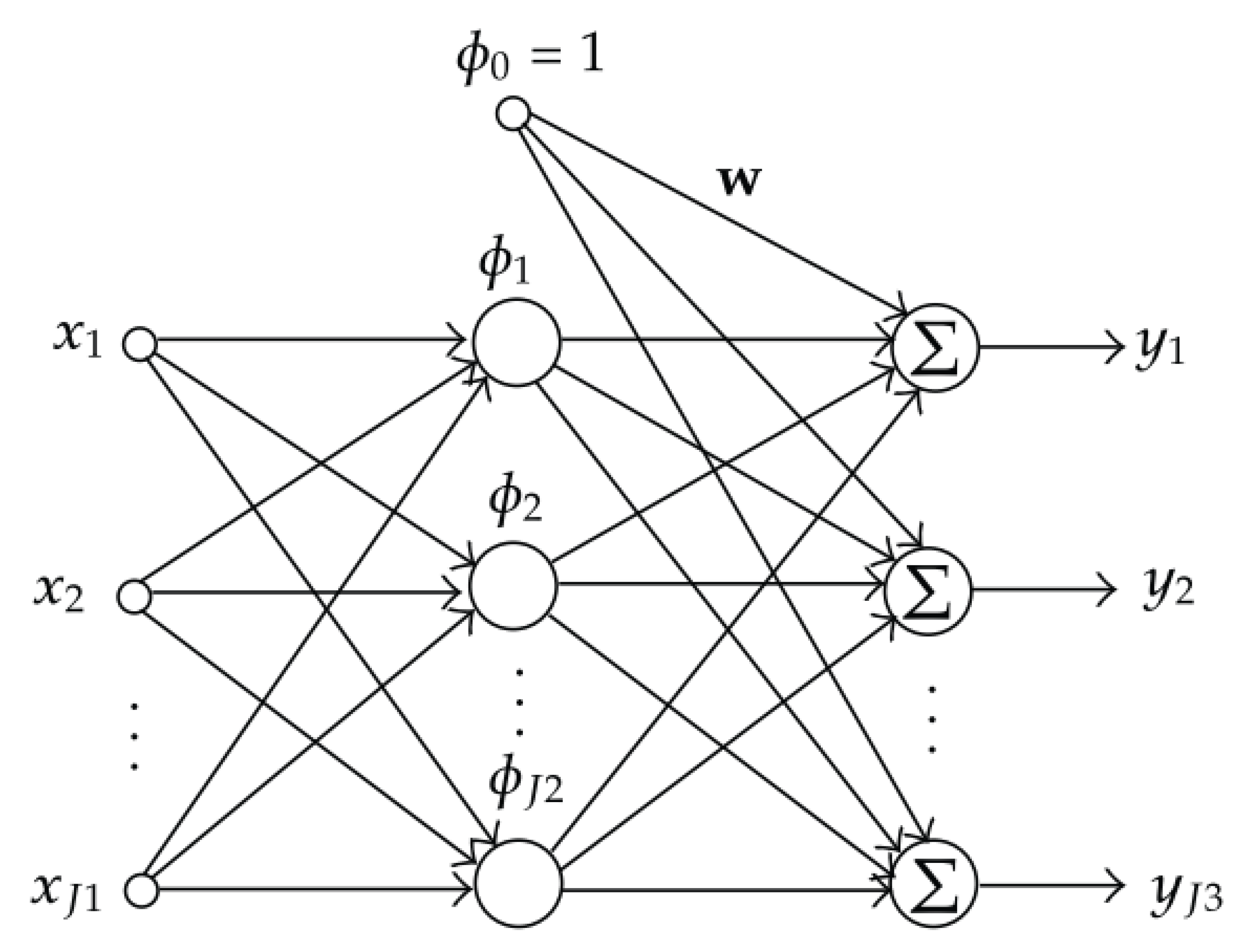
Figure 1. Architecture of the RBF network. The input, hidden and output layers have J1, J2 and J3 neurons, respectively ^[6].

1.3. Autoencoders

The autoencoder is a particular feedforward neural network trained using unsupervised learning. The autoencoder learns to reproduce the unit mapping from a certain information input vector

\vec{I} \in R^{n \times n}

\vec{I}

itself. The topological constraint dictates that the number of neurons in the next layer must be lower than the previous one. Such a constraint forces the network to learn a description of the input vector that belongs to the lower-dimensional space of the subsequent layers without losing information. The amount of information lost while encoding a downsizing the input vector is measured by the fitting discrepancy between the input and the reconstructed vector

\vec{I}

^[7]^[8]^[9]. The desired lower-dimensional vector concentrating the information contained in the input vector is the layer at which the network starts growing again; see Figure 2. It is important to note that the structure of an autoencoder is exactly the same as the MLP, with the additional constraint of having the same numbers of input and output nodes.

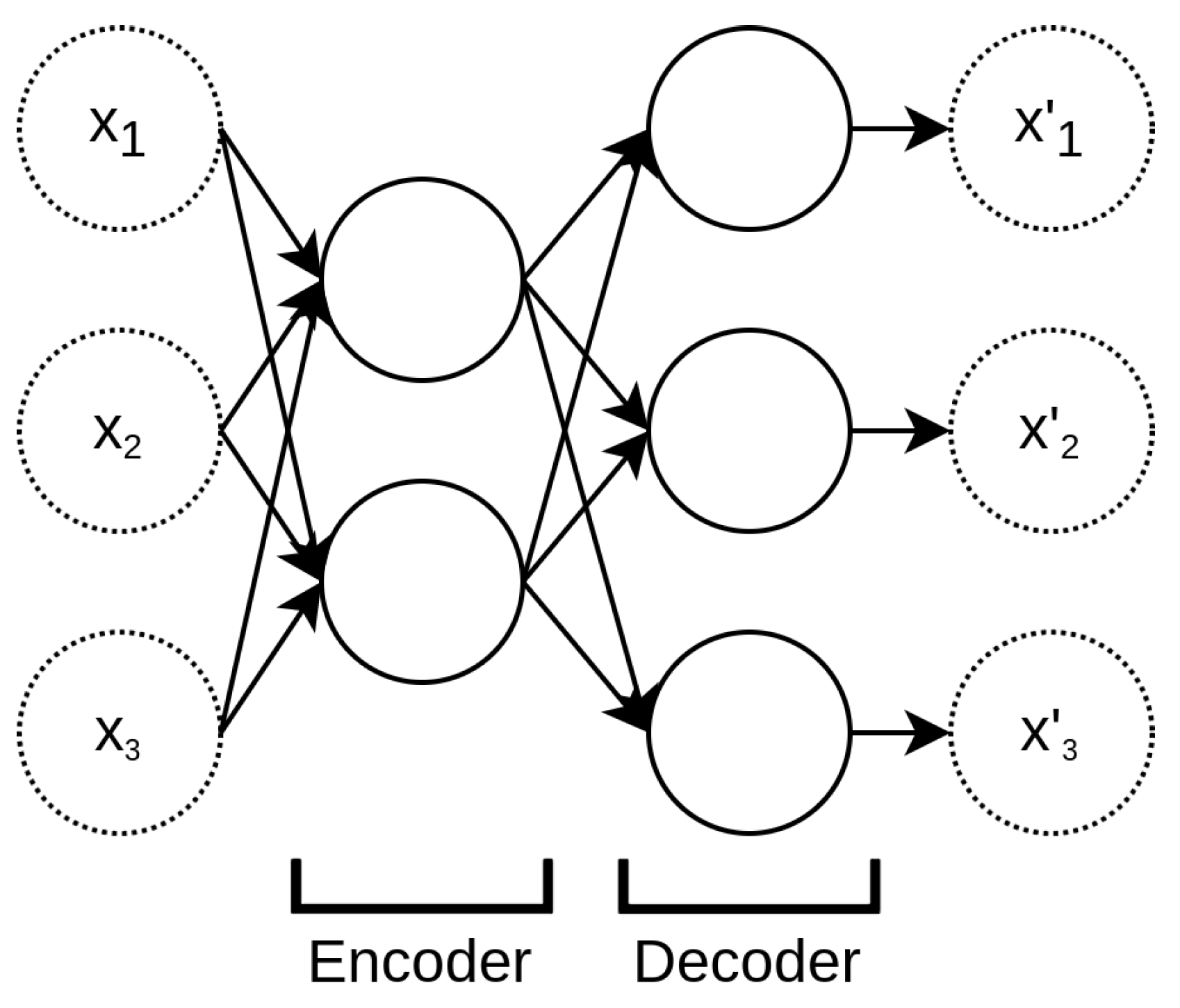
Figure 2. Basic autoencoder structure.

The autoencoders are widely used for unsupervised applications: typically, they are used for denoising, dimensionality reduction and data representation learning.

1.4. Convolutional Neural Networks

Feedforward networks are of extreme importance to machine learning applications in the space domain. A specialized kind of feedforward network, often referred as a stand-alone type, is the convolutional neural network (CNN) ^[10]. Convolutional networks are specifically tailored for image processing; for instance, CNNs are used for object recognition, image segmentation and classification. The main reason why traditional feedforward networks are not suitable for handling images is due to the fact that one image can be thought of as a large matrix array. The number of weights, or parameters, to efficiently process large two-dimensional images (or three if more image channels are involved) quickly explodes as the image resolution grows. In general, given a network of width W and depth D, the number of parameters

n_{w}

for a fully connected network is

n_{w} \sim D W^{2} + W

. For instance, a low resolution image

\vec{I} \in R^{32 \times 32}

has a width of

W^{2}

, by simply unrolling the image into a 1D array: this means that

n_{w} 10^{6}

. A high resolution image, e.g.,

\vec{I} \in R^{1024 \times 1024}

, quickly reaches

n_{w} \sim 10^{12}

. This shortcoming results in complex training procedures, very much subject to overfitting. The convolutional neural network paradigm stands for the idea of reducing the number of parameters starting from the main assumptions:

Low-level features are local;
Features are translationally invariant;
High-level features are composed of low-level features.

Such assumptions allow a reduction in the number of parameters while achieving better generalization and improved scalability to large datasets. Indeed, instead of using fully connected layers, a CNN uses local connectivity between neurons; i.e., a neuron is only connected to nearby neurons in the next layer ^[8]. The basic components of a convolutional neural network are:

Convolutional layer: the convolutional layer is core of the CNN architecture. The convolutional layer is built up by neurons which are not connected to every single neuron from the previous layer but only to those falling inside their receptive field. Such architecture allows the network to identify low-level features in the very first hidden layer, whereas high-level features are combined and identified at later stages in the network. A neuron’s weight can be thought of as a small image, called the filter or convolutional kernel, which is the size of the receptive field. The convolutional layer mimics the convolution operation of a convolutional kernel on the input layer to produce an output layer, often called the feature map. Typically, the neurons that belong to a given convolutional layer all share the same convolutional kernel: this is referred to as parameter sharing in the literature. For this reason, the element-wise multiplication of each neuron’s weight by its receptive field is equivalent to a pure convolution in which the kernel slides across the input layer to generate the feature map. In mathematical terms, a convolutional layer, with convolutional kernel $\vec{W}$ , operating on the previous layer $\vec{I}$ (being either an intermediate feature map or the input image), performs the following operation:

$f_{i, j} = (\vec{I} * \vec{W})$

where $f_{i, j}$ is the $(i, j)$ position of the output feature map.
Activation layer: An activation function is utilized as a decision gate that aids the learning process of intricate patterns. The selection of an appropriate activation function can accelerate the learning process ^[10]. The most common activation functions are the same as those used for the MLP and are presented.
Pooling layer: The objective of a pooling layer is to sub-sample the input image or the previous layer in order to reduce the computational load, the memory usage and the number of parameters, which prevents overfitting while training ^[10]^[11]. The pooling layer works exactly with the same principle of the receptive field. However, a pooling neuron has no weights; hence, it aggregates the inputs by calculating the maximum or the average within the receptive field as output.
Fully-connected layer: Similarly to MLP as for traditional CNN architectures, a fully connected layer is often added right before the output layer to further capture non-linear relationships of the input features ^[8]^[10]. The same considerations discussed for MLP hold for CNN fully connected layers.

An example of a CNN architecture is shown in Figure 3.

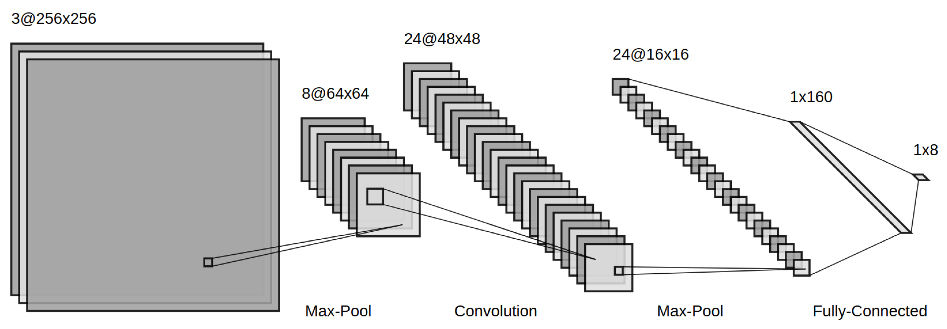
Figure 3. Example CNN architecture with convolutional, max-pooling and fully connected layers.

2. Recurrent Neural Networks

Recurrent neural networks comprise all the architectures that present at least one feedback loop in their layer interactions ^[1]. A subdivision that is seldom used is between finite and infinite impulse recurrent networks. The former is given by a directed acyclic graph (DAG) that can be unrolled in time and replaced with a feedforward neural network. The latter is a directed cyclic graph (DCG) that cannot be unrolled and replaced similarly ^[8]. Recurrent neural networks have the capability of handling time-series data efficiently. The connections between neurons form a directed graph, which allows internal state memory. This enables the network to exhibit temporal dynamic behaviors.

2.1. Layer-Recurrent Neural Network

The core of the layer-recurrent neural network (LRNN) is similar to that of the standard MLP ^[1]. This means that the same considerations for model depth, width and activation functions hold in the same manner. The only addition is that in the LRNN, there is a feedback loop with a single delay around each layer of the network, except for the last layer. A schematic of the LRNN is sketched in Figure 4.

Figure 4. Schematic of a layer-recurrent neural network. The feedback loop is a tap-delayed signal rout.

2.2. Nonlinear Autoregressive Exogenous Model

The nonlinear autoregressive exogenous model is an extension of the LRNN that uses the feedback coming from the output layer ^[12]. The LRNN owns dynamics only at the input layer. The nonlinear autoregressive network with exogenous inputs (NARX) is a recurrent dynamic network with feedback connections enclosing several layers of the network. The NARX model is based on the linear ARX model, which is commonly used in time-series modeling. The defining equation for the NARX model is

y_{k} = N (y_{k - 1}, y_{k - 2}, \dots, y_{k - n}, u_{k - 1}, u_{k - 2}, \dots, u_{k - n})

where y is the network output and u is the exogenous input, as shown in Figure 5. Basically, it means that the next value of the dependent output signal y is regressed on previous values of the output signal and previous values of an independent (exogenous) input signal. It is important to remark that, for a one tap-delay NARX, the defining equation takes the form of an autonomous dynamical system.

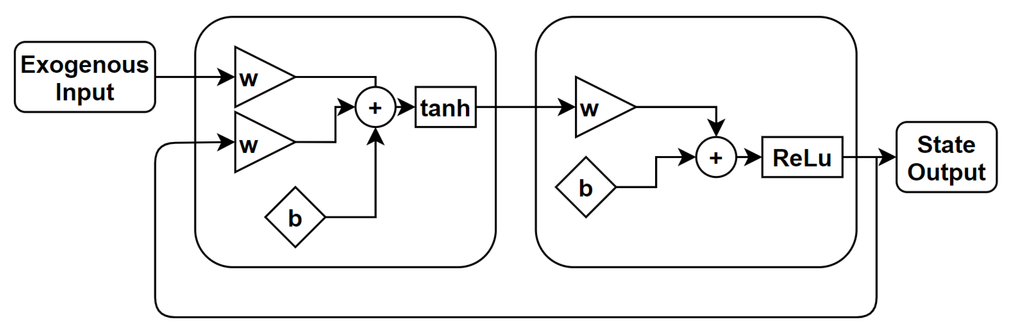
Figure 5. Schematic of a nonlinear autoregressive exogenous model. The feedback loop is a tap-delayed signal rout ^[13].

2.3. Hopfield Neural Network

The formulation of the network was due to Hopfield ^[14], but the formulation by Abe ^[15] is reportedly the most suited for combinatorial optimization problems ^[16], which are of great interest in the space domain. For this reason, here the most recent architecture is reported. A schematic of the network architecture is shown in Figure 6.

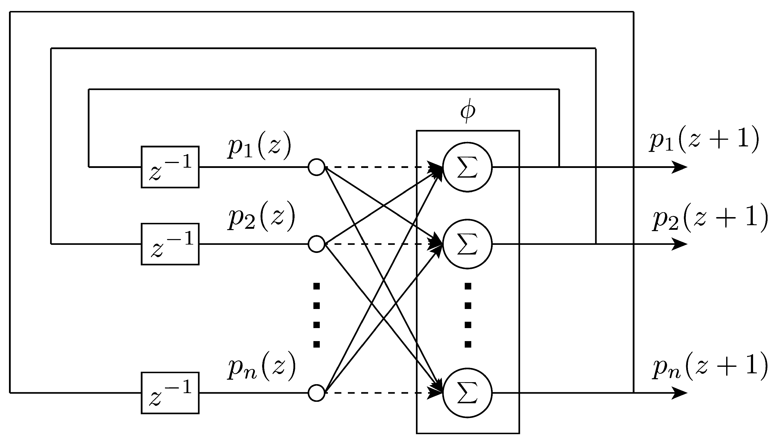
Figure 6. The Hopfield neural network structure ^[16].

In synthesis, the dynamics of the i-th out of N neurons is written as:

\frac{d p_{i}}{d t} = \sum_{j = 1}^{N} w_{i j} s_{j} - b_{i}

where

p_{i}

is the total input of the i-th neuron;

w_{i j}

and

b_{i}

are parameters corresponding, respectively, to the synaptic efficiency associated with the connection from neuron j to neuron i and the bias of the neuron i. The term

s_{i}

is basically the equivalent of the activation function:

s_{i} = c_{i} tanh \frac{p_{i}}{β}

where

β > 0

is a user-defined coefficient, and

c_{i}

is the user-defined amplitude of the activation function. The recurrent structure of the network entails the dynamics of the neurons; hence, it would be more correct to refer to

p (t)

and

s (t)

as functions of time or any other independent variable. An important property of the network, which will be further discussed in the application for parameter identification, is that the Lyapunov stability theorem can be used to guarantee its stability. Indeed, since a Lyapunov function exists, the only possible long-term behavior of the neurons is to asymptotically approach a point that belongs to the set of fixed points, meaning where

\frac{d V}{d t} = 0

V

being the Lyapunov function of the system, in the form:

V = - \frac{1}{2} \sum_{i = 1}^{N} \sum_{j = 1}^{N} w_{i j} s_{i} s_{j} + \sum_{i = 1}^{N} b_{i} s_{i} = - \frac{1}{2} {\vec{s}}^{T} W \vec{s} + {\vec{s}}^{T} \vec{b}

where the right-hand term is expressed in a compact form, with

\vec{s}

, the vector of s neuron states, and

\vec{b}

, the bias vector. A remarkable property of the network is that the trajectories always remain within the hypercube

[- c_{i}, c_{i}]

as long as the initial values belong to the hypercube too ^[16]^[17]. For implementation purposes, the discrete version of the HNN is employed, as was done in ^[16]^[18].

2.4. Long Short-Term Memory

The long-short term memory network is a type of recurrent neural network widely used for making predictions based on times series data. LSTM, first proposed by Hochreiter ^[19], is a powerful extension of the standard RNN architecture because it solves the issue of vanishing gradients, which often occur in network training. In general, the repeating module in a standard RNN contains a single layer. This means that if the RNN is unrolled, you can replicate the recurrent architecture by juxtaposing a single layer of nuclei. LSTMs can also be unrolled, but the repeating module owns four interacting layers or gates. The basic LSTM architecture is shown in Figure 7.

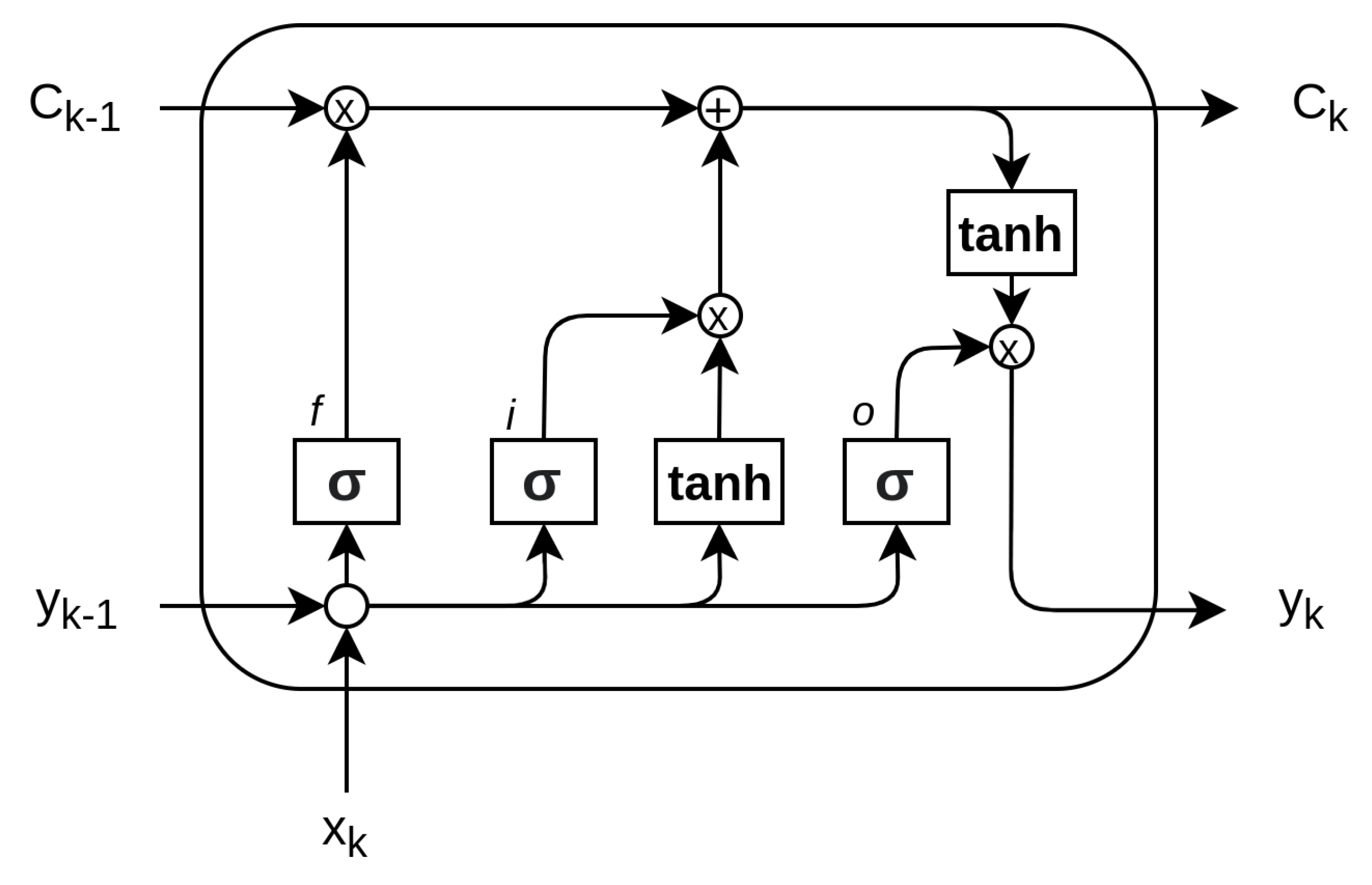
Figure 7. The core components of the LSTM are the cell (C), the input gate (i), the output gate (o) and the forget gate (f) ^[19].

The core idea is that the cell state lets the information flow: it is modified by the three gates, composed of a sigmoid neural net layer and a point-wise multiplication operation. The sigmoid layer of each gate outputs a value

\in [0, 1]

that defines how much of the core information is let through. The basic components of the LSTM network are summarized here:

Cell state (C): The cell state is the core element. It conveys information through different time steps. It is modified by linear interactions with the gates.
Forget gate (f): The forget gate is used to decide which information to let through. It looks at the input $x_{k}$ and output of the previous step $y_{k - 1}$ and yields a number $\in [0, 1]$ for each element of the cell state. In compact form:

$f = σ (W_{f} \cdot [y_{k - 1}, x_{k}] + {\vec{b}}_{f}]$
Input gate (i): The input gate is used to decide what piece of information to include in the cell state. The sigmoid layer is used to decide on which value to update, whereas the $t a n h$ describes the entities for modification, namely, the values. It then generates a new estimate for the cell state $\tilde{C}$ :

$\begin{matrix} i & = σ (W_{i} \cdot [y_{k - 1}, x_{k}] + {\vec{b}}_{i}) \\ {\tilde{C}}_{k} & = tanh (W_{c} \cdot [y_{k - 1}, x_{k}] + {\vec{b}}_{c}) \end{matrix}$
Memory gate: The memory gate multiplies the old cell state with the output of the forget gate and adds it to the output of the input gate. Often, the memory gate is not reported as a stand-alone gate, due to the fact that it represents a modification of the cell state itself, without a proper sigmoid layer:

$C_{k} = f ⊙ C_{k - 1} + i ⊙ {\tilde{C}}_{k}$
Output gate: The output gate is the final step that delivers the actual output of the network $y_{k}$ , a filtered version of the cell state. The layer operations read:

$\begin{matrix} o & = σ (W_{o} \cdot [y_{k - 1}, x_{k}] + {\vec{b}}_{o}) \\ y_{k} & = o ⊙ tanh C_{k} \end{matrix}$

In contrast to deep feedforward neural networks, having a recurrent architecture, LSTMs contain feedback connections. Moreover, LSTMs are well suited not only for processing single data points, such as input vectors, but efficiently and effectively handle sequences of data. For this reason, LSTMs are particularly useful for analyzing temporal series and recurrent patterns.

2.5. Gated Recurrent Unit

The gated recurrent unit (GRU) was proposed by Cho ^[20] to make each recurrent unit adaptively capture dependencies of different time scales. Similarly to the LSTM unit, the GRU has gating units that modulate the flow of information inside the unit, but without having a separate memory cells ^[20]^[21]. The basic components of GRU share similarities with LSTM. Traditionally, different names are used to identify the gates:

Update gate (u): The update gate defines how much the unit updates its value or content. It is a simple layer that performs:

$u = σ (W_{u} \cdot [y_{k - 1}, x_{k}] + {\vec{b}}_{u})$
Reset gate r: The reset gate effectively makes the unit process the input sequence, allowing it to forget the previously computed state:

$r = σ (W_{r} \cdot [y_{k - 1}, x_{k}] + {\vec{b}}_{r})$

The output of the network is calculated through a two-step update, entailing a candidate update activation

{\tilde{y}}_{k}

calculated in the activation h layer and the output

y_{k}

\begin{matrix} {\tilde{y}}_{k} & = tanh W_{h} \cdot [y_{k - 1}, x_{k}] + {\vec{b}}_{h} \\ y_{k} & = (1 - u) ⊙ y_{k - 1} + u ⊙ {\tilde{y}}_{k} \end{matrix}

A schematic of GRU network is reported in Figure 8.

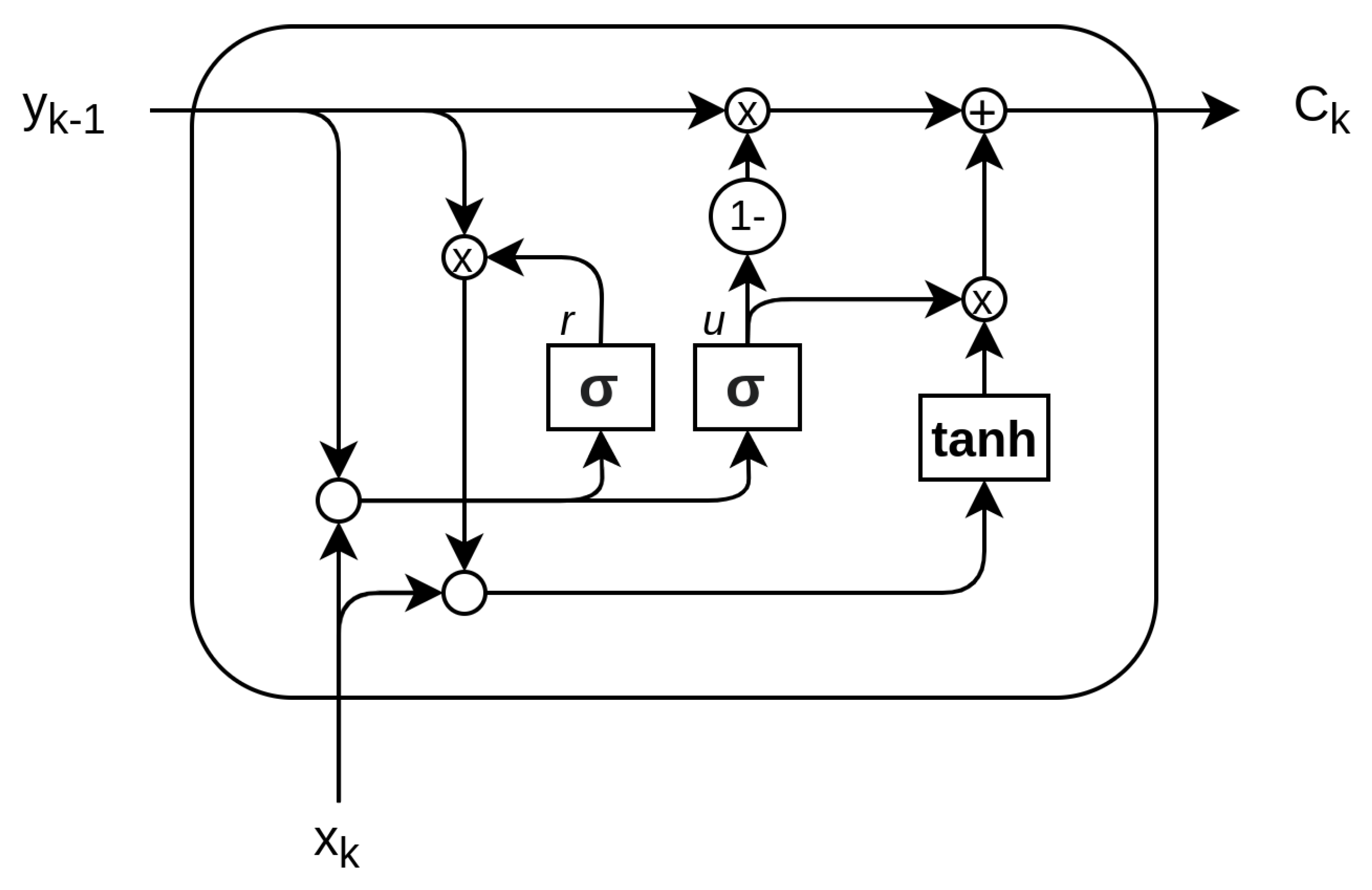
Figure 8. The core components of the GRU are the reset gate (r) and the update gate (u) coupled with the activation output composed of the

tanh

layer.

3. Spiking Neural Networks

Spiking neural networks (SNN) are becoming increasingly interesting to the space domain due to their low-power and energy efficiency. Indeed, small satellite missions entail low-computational-power devices and in general lower system power budgets. For this reason, SNNs represent a promising candidate for the implementation of neural-based algorithms used for many machine learning applications: among those, the scene classification task is of primary importance for the space community. SNNs are the third generation of artificial neural networks (ANNs), where each neuron in the network uses discrete spikes to communicate in an event-based manner. SNNs have the potential advantage of achieving better energy efficiency than their ANN counterparts. While generally a loss of accuracy in SNN models is reported, new algorithms and training techniques can help with closing the gap in accuracy performance while keeping the low-energy profile. Spiking neural networks (SNNs) are inspired by information processing in biology. The main difference is that neurons in ANNs are mostly non-linear but continuous function evaluations that operate synchronously. On the other hand, biological neurons employ asynchronous spikes that signal the occurrence of some characteristic events by digital and temporally precise action potentials. In recent years, researchers from the domains of machine learning, computational neuroscience, neuromorphic engineering and embedded systems design have tried to bridge the gap between the big success of DNNs in AI applications and the promise of spiking neural networks (SNNs) ^[22]^[23]^[24]. The large spike sparsity and simple synaptic operations (SOPs) in the network enable SNNs to outperform ANNs in terms of energy efficiency. Nevertheless, the accuracy performance, especially in complex classification tasks, is still superior for deep ANNs. In the space domain, the SNNs are at the earliest stage of research: mission designers strive to create algorithms characterized by great computational efficiency and low power applications; although they are not yet applied to guidance, navigation and control applications. Finally, SNNs on neuromorphic hardware exhibit favorable properties such as low power consumption, fast inference and event-driven information processing. This makes them interesting candidates for the efficient implementation of deep neural networks particularly utilized in image classification.

The most peculiar feature of SNNs is that the neurons possess temporal dynamics: typically, an electrical analogy is used to describe their behavior. Each neuron has a voltage potential that builds up depending on the input current that it receives. The input current is generally triggered by the spikes the neuron receives. A schematic of the neuron parameters can be seen in Figure 9 and Figure 10. There are numerous neural architectures that combine these notions into a set of mathematical equations; nevertheless, the two most common alternatives are the integrate-and-fire neuron and the leaky-integrate-and-fire neuron.

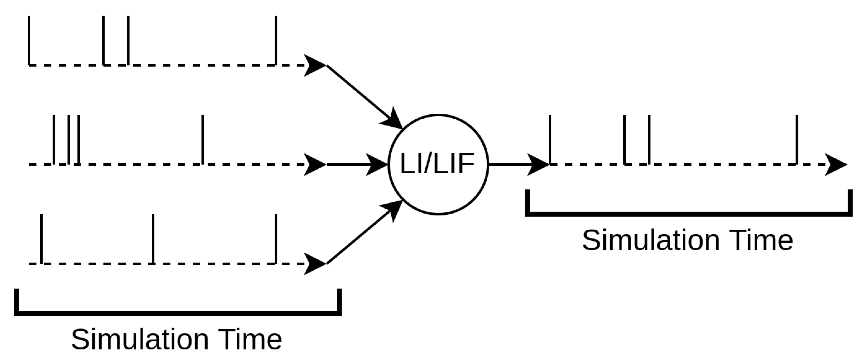
Figure 9. Architecture of a simple spiking neuron. Spikes are received as inputs, which are then either integrated or summed depending on the neuron model. The output spikes are generated when the internal state of the neuron reaches a given threshold.

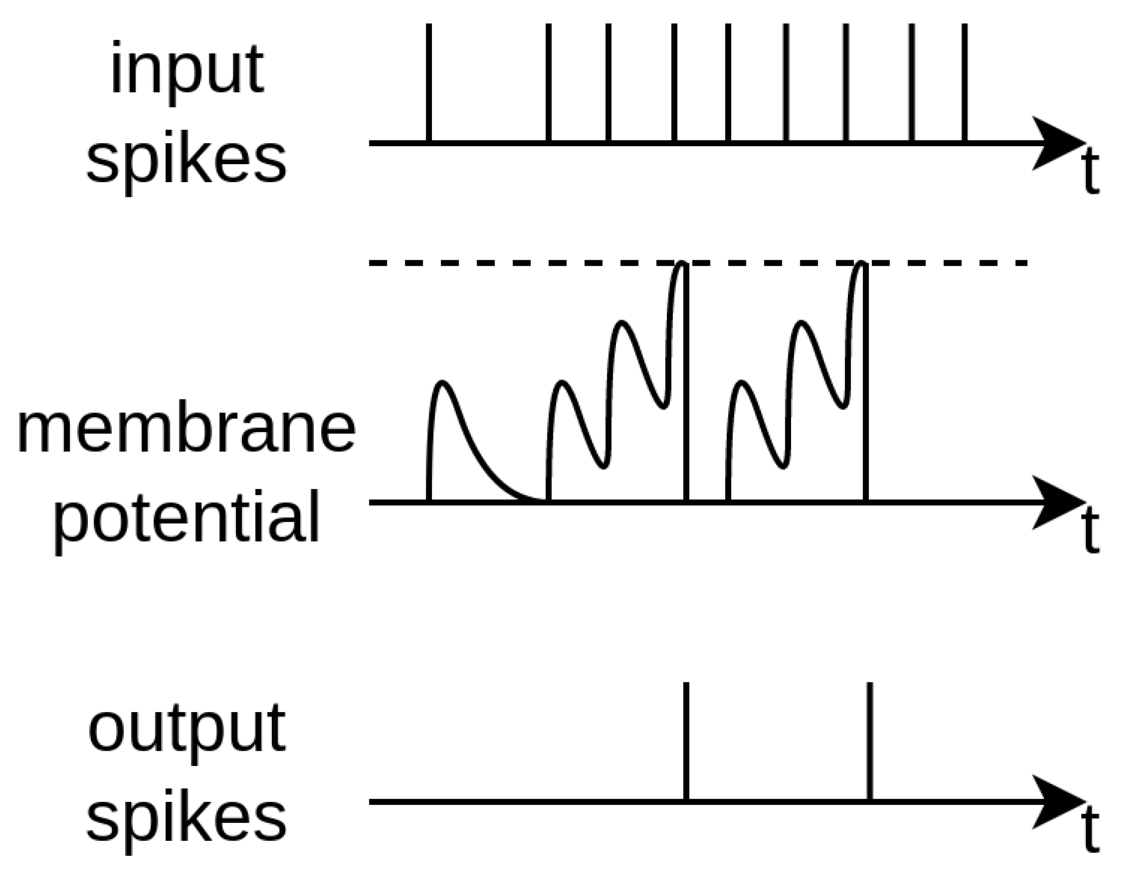
Figure 10. An illustrative schematic depicting the membrane potential reaching the threshold, which generates output spikes ^[23].

3.1. Types of Neurons

Integrate and fire (IF): The IF neuron model assumes that spike initiation is governed by a voltage threshold. When the synaptic membrane reaches and exceeds a certain threshold, the neuron fires a spike and the membrane is set back to the resting voltage $V_{r e s t}$ . In mathematical terms, its simplest form reads:

$C \frac{d V (t)}{d t} = i (t)$
Leaky integrate and fire (LIF): The LIF neuron is a slightly modified version of the IF neuron model. Indeed, it entails an exponential decrease in membrane potential when not excited. The membrane charges and discharges exponentially in response to injected current. The differential equation governing such behavior can be written as:

$C \frac{d V (t)}{d t} + λ V (t) = i (t)$

where $λ$ is the leak conductance and V is again the membrane potential with respect to the rest value.

As mentioned, the list is not extensive, and the reader is suggested to refer to ^[25] for a comprehensive review of neuron models.

3.2. Coding Schemes

The transition between dense data and sparse spiking patterns requires a coding mechanism for input coding and output decoding. For what concerns the input coding, the data can be transformed from dense to sparse spikes in different ways, among which the most used are:

Rate coding: it converts the input intensity into a firing rate or spike count;
Temporal (or latency) coding: it converts the input intensity to a spike time or relative spike time.

Similarly, in output decoding, the data can be transformed from sparse spikes to network output (such as classification class) in different ways, among which the most used are:

Rate coding: it selects the output neuron with the highest firing rate, or spike count, as the predicted class;
Temporal (or latency) coding: it selects the output neuron that fires first, or before a given threshold time, as the predicted class

Roughly speaking, the current literature agrees on specific advantages for both the coding techniques. On one hand, the rate coding is more error tolerant given the reduced sparsity of the neuron activation. Moreover, the accuracy and learning convergence have shown superior results in rate-based applications so far. On the other hand, given the inherent sparsity of the encoding-decoding scheme, latency-based approaches tend to outperform the rate-based architectures in inference, training speed and, above all, power consumption.

References

Goodfellow, I.; Bengio, Y.; Courville, A. Deep Learning; Massachusetts Institute of Technology: Massachusetts, MA, USA, 2016.
Fausett, L. Fundamentals of Neural Networks; Pearson: London, UK, 1994.
Lippmann, R. Neural Networks, a Comprehensive Foundation; Prentice Hall: Hoboken, NJ, USA, 2005; Volume 5, pp. 363–364.
Silvestrini, S.; Lavagna, M. Neural-aided GNC reconfiguration algorithm for distributed space system: Development and PIL test. Adv. Space Res. 2021, 67, 1490–1505.
Pesce, V.; Silvestrini, S.; Lavagna, M. Radial basis function neural network aided adaptive extended Kalman filter for spacecraft relative navigation. Aerosp. Sci. Technol. 2020, 96, 105527.
Wu, Y.; Wang, H.; Zhang, B.; Du, K.L. Using Radial Basis Function Networks for Function Approximation and Classification. ISRN Appl. Math. 2012, 2012, 1–34.
Shrestha, A. Review of Deep Learning Algorithms and Architectures. IEEE Access 2019, 7, 53040–53065.
Emmert-Streib, F.; Yang, Z.; Feng, H.; Tripathi, S.; Dehmer, M. An Introductory Review of Deep Learning for Prediction Models With Big Data. Front. Artif. Intell. 2020, 3, 1–23.
Masti, D.; Bemporad, A. Learning Nonlinear State-Space Models Using Deep Autoencoders. In Proceedings of the IEEE Conference on Decision and Control, Paris, France, 11–13 December 2019; Volume 2018-12, pp. 3862–3867.
Khan, A.; Sohail, A.; Zahoora, U.; Saeed, A. A Survey of the Recent Architectures of Deep Convolutional Neural Networks; Springer: Amsterdam, The Netherlands, 2020; Volume 53, pp. 5455–5516.
Géron, A. Hands-On Machine Learning with Scikit-Learn, Keras, and TensorFlow; O’Reilly Media: Sebastopol, CA, USA, 2019.
Nelles, O. Nonlinear System Identification; Springer: London, UK, 2003; Volume 39, pp. 564–568.
Silvestrini, S.; Lavagna, M. Relative Trajectories Identification in Distributed Spacecraft Formation Collision-Free Maneuvers using Neural-Reconstructed Dynamics. In Proceedings of the AIAA Scitech 2020 Forum, Kissimmee, FL, USA, 8–12 January 2020; pp. 1–14.
Hopfield, J.J. Neurons with graded response have collective computational properties like those of two-state neurons. Proc. Natl. Acad. Sci. USA 1984, 81, 3088–3092.
Abe. Theories on the Hopfield neural networks. In Proceedings of the International 1989 Joint Conference on Neural Networks, Washington, DC, USA, 6 August 1989; Volume 1, pp. 557–564.
Pasquale, A.; Silvestrini, S.; Capannolo, A.; Lavagna, M. Non-Uniform Gravity Field Model On-Board Learning During Small Bodies Proximity Operations. In Proceedings of the 70th International Astronautical Congress, Washington, DC, USA, 21–25 October 2019; pp. 21–25.
Atencia, M.; Joya, G.; Sandoval, F. Parametric identification of robotic systems with stable time-varying Hopfield networks. Neural Comput. Appl. 2004, 13, 270–280.
Hernández-Solano, Y.; Atencia, M.; Joya, G.; Sandoval, F. A Discrete Gradient Method to Enhance the Numerical Behaviour of Hopfield Networks. Neurocomputers 2015, 164, 45–55.
Hochreiter, S.; Schmidhuber, J. Long Short-Term Memory. Neural Comput. 1997, 9, 1735–1780.
Cho, K.; van Merriënboer, B.; Gulcehre, C.; Bahdanau, D.; Bougares, F.; Schwenk, H.; Bengio, Y. Learning Phrase Representations using RNN Encoder–Decoder for Statistical Machine Translation. In Proceedings of the 2014 Conference on Empirical Methods in Natural Language Processing (EMNLP), Doha, Qatar, 25–29 October 2014; Association for Computational Linguistics: London, UK, 2014; pp. 1724–1734.
Chung, J.; Gulcehre, C.; Cho, K.; Bengio, Y. Empirical evaluation of gated recurrent neural networks on sequence modeling. In Proceedings of the NIPS 2014 Workshop on Deep Learning, Montreal, BC, Canada, 12 December 2014.
Ponulak, F.; Kasiński, A. Information Processing, Learning and Applications; Springer: Amsterdam, The Netherlands, 2011; pp. 409–433.
Eshraghian, J.K.; Ward, M.; Neftci, E.; Wang, X.; Lenz, G.; Dwivedi, G.; Bennamoun, M.; Jeong, D.S.; Lu, W.D. Training Spiking Neural Networks Using Lessons from Deep Learning; Cornell University: Ithaca, NY, USA, 2021; pp. 1–44.
Pfeiffer, M.; Pfeil, T. Deep Learning With Spiking Neurons: Opportunities and Challenges. Front. Neurosci. 2018, 12, 774.
Nguyen, D.A.; Tran, X.T.; Iacopi, F. A review of algorithms and hardware implementations for spiking neural networks. J. Low Power Electron. Appl. 2021, 11, 23.

© Text is available under the terms and conditions of the Creative Commons Attribution (CC BY) license; additional terms may apply. By using this site, you agree to the Terms and Conditions and Privacy Policy.

Upload a video for this entry

Information

Subjects: Engineering, Aerospace

Contributors MDPI registered users' name will be linked to their SciProfiles pages. To register with us, please refer to https://encyclopedia.pub/register :

Stefano Silvestrini

Michèle Lavagna

View Times: 1.5K

Update Date: 27 Sep 2022

Table of Contents

Video Upload Options

Confirm

1. Feed-Forward Networks

1.1. Multilayer Perceptron

1.2. Radial-Basis Function Neural Network

1.3. Autoencoders

1.4. Convolutional Neural Networks

2. Recurrent Neural Networks

2.1. Layer-Recurrent Neural Network

2.2. Nonlinear Autoregressive Exogenous Model

2.3. Hopfield Neural Network

2.4. Long Short-Term Memory

2.5. Gated Recurrent Unit

3. Spiking Neural Networks

3.1. Types of Neurons

3.2. Coding Schemes

References