Machine Learning for Crop Diseases and Pests

Version	Summary	Created by	Modification	Content Size	Created at	Operation
1		Tiago Domingues	--	6316	2022-09-15 17:04:32	\|
2	Format correction	Sirius Huang	Meta information modification	6316	2022-09-16 03:53:57	\|

This entry is adapted from the peer-reviewed paper 10.3390/agriculture12091350

Rapid population growth has resulted in an increased demand for agricultural goods. Pests and diseases are major obstacles to achieving this productivity outcome. Therefore, it is very important to develop efficient methods for the automatic detection, identification, and prediction of pests and diseases in agricultural crops. To perform such automation, Machine Learning (ML) techniques can be used to derive knowledge and relationships from the data that is being worked on.

plant diseases and pests classification detection forecasting precision farming machine learning smart farming

1. Introduction

Machine learning (ML)-based applications for agriculture are still young, but are already showing promise. For instance, disease classification from images can be done using popular Convolutional Neural Network (CNN) architectures for different plants with different diseases ^[1]; relationships between weather data and pest occurrence can be retrieved using Long Short Term Memory (LSTM) networks for forecasting future pest attacks ^[2]; insect detection on leaves can be performed using object segmentation and deep learning techniques ^[3].

Data gathering, data pre-processing (i.e., data preparation that includes feature extraction), and ML classification models are the three basic steps of ML applications, represented in Figure 1. The following sections present and discuss different approaches used in these three stages.

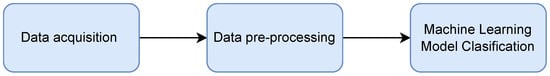
Figure 1. Simplification of the ML pipeline.

2. Data Acquisition

Data acquisition is the process of gathering data from various sources systems ^[4]. Previous studies gather their data various sources to be used for ML techniques. Some of them produce their own images by taking pictures of plants in greenhouses, such as in the studies from Gutierrez et al. ^[3] and Raza et al. ^[5]. However, image data acquisition using manual processes, as done by many, generally results in small image data-sets, which can compromise the development of effective ML-based models. Weather data collection is also proposed in the literature using for instance sensors in greenhouses, as done by Rustia and Lin ^[6]. Meteorological data can also be obtained from weather stations of regional areas, which typically store records for a longer period of time ^[2]^[7].

Images can be collected using search engines on their own ^[8]^[9]. This approach can get a large number of images, but ground truth must be checked by domain experts, and data cleaning is frequently used to filter out images that do not meet the requirements.

Remote sensing images from satellites and drones have the advantage of being able to retrieve image data for large agricultural areas. Remote sensing data from satellites typically consists of multi-temporal and hyper-spectral imagery data, which can be used to assess the development of the crops. This task can be performed by monitoring the evolution of vegetation indices ^[10], which provide important information about the development status of the crop fields. Spectral imagery can be used for computing different vegetation indexes, such as those proposed in ^[11]^[12]^[13]^[14]^[15]^[16]^[17], which are robust to variations on the sun illumination ^[15], an important advantage when compared to visible light spectrum imagery.

Images retrieved from drones can also be used, but have additional needs: to define the path of the device; to coordinate the drone position with the camera for image acquisition; and to correct geometric distortions on each acquired image in order to merge the different acquired images in order to reconstruct a larger image of the whole field ^[18].

2.1. Variables Influencing Crop Diseases and Pests

It’s crucial to be able to predict the arrival of diseases and pests in crops, in addition to correctly detecting and identifying them. Real-time meteorological data obtained by unmanned observation planes, as well as long-term data analysis from weather stations, have been used to create models capable of anticipating disease occurrence. In ^[19], the General Infection Model, proposed in ^[20], was used for assessing the prediction capabilities of the system. It was found that, if integrated systems such as this are implemented and various input data-sets essential for interrelationship analyses are collected, accurate plant disease prediction systems can be constructed.

When it comes to forecasting occurrences, it’s crucial to know which variables will have an influence on what is being forecast. In the work by Henderson et al. ^[21] this was done by discovering which weather variables influence the forecast. On the other hand, Lasso et al. ^[22] determined the time period window for each weather variable and crop-related feature that is the most significant for the appearance of coffee leaf rust disease in coffee crops.

In ^[23], Small et al. used weather data, information on potato and tomato crops resistance to late blight (from published literature and field experiments), and management strategies, to create a web-based decision support system that allows the dynamic prediction of disease outbreaks, with an emphasis on the late blight disease on tomato and potato crops.

The work proposed by Ghaffari et al. ^[24] addresses the very early detection of diseases in tomato crops using atmospheric data and volatile organic compounds. Plants produce a wide spectrum of volatile organic compounds in reaction to physical and biotic stress, as well as infection ^[25]. In ^[24], the diseases under study were the powdery mildew and spider mites.

A model developed by Diepeveen et al. in ^[26] can be used in agriculture to understand the influence of location and temperature on crops. In addition, elements such as soil, humidity, rainfall, and moisture were found to have an influence on crop yield ^[27].

Plant diseases and pest development are greatly influenced by weather and environment conditions ^[28]. Humidity is a favorable condition for the development of fungus diseases. The humidity can be caused by the weather or by poor watering practices that cause a high wetness among the leaves, making tomatoes more susceptible to diseases, e.g., leaf mold or bacterial spot ^[29].

In addition, temperature is a primary driver of insect development, affecting their metabolic rate and population growth ^[30].

Plants absorb part of the radiation coming from the sun and reflect the rest. Depending on the health of the plant, the amount of radiation absorbed and reflected differs. This difference can be used to distinguish between healthy and diseased plants and to assess the severity of the damage ^[31]. The concept is illustrated in Figure 2.

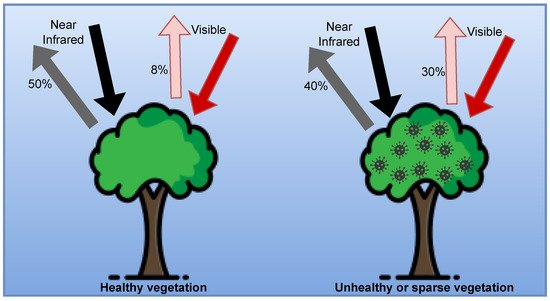
Figure 2. Absorbed and reflected radiation for plant’s health estimation (adapted from ^[32]).

Temperature

Insects are ectothermic, meaning that they cannot regulate their internal temperature and have to rely on environmental heat sources. Temperature affects the population growth and metabolic rates of insects ^[30]. Thus, the duration of an insect’s life cycle is highly influenced by the number of days where the temperature is suitable for its development. Two temperature thresholds can be define: an upper threshold, in which insect development slows down or stops and a lower one where there is no insect growth. These thresholds vary according to the specific insect species.

Degree day is a concept concerning the accumulation of heat by insects ^[33]. One degree day is a period of 24 h in which the temperature was one degree above a given baseline. Different models for determining the number of degree days associated to common pest species were proposed in ^[34]. For instance, tomato crops are susceptible to the greenhouse white fly (Trialeurodes vaporariorum), whose number of degree days from egg to adult is 380 DGG ^[35]. Depending on the temperature of the environment, this development time can be longer or shorter.

Biofix date is the date to start accumulating degree days associated with a given insect species ^[36]. This date can be determined by noticing specific insect species on traps or by detecting eggs on plant leaves. From this date, degree days can be used to estimate the period at which insects are reaching a given development stage suitable for pesticide application. Temperature and weather forecasts are nowadays sufficiently accurate to enable the estimation for the time required for an insect to reach a given development status ^[37].

In the context of ML-based applications, related work focused on studying the impact of weather in pest insect development found a higher correlation between the number of pest catches and temperature, when compared with other factors ^[6]^[10].

Some diseases affect the transpiration rate of the plant and, consequently, its temperature ^[5]. Therefore, plant leaf temperature can be used for disease detection. ML models can achieve higher accuracy for disease identification when combining thermal images with visible light images. The benefits are more useful for early detection when the plant has not yet developed symptoms recognizable by the naked eye.

Humidity

Diseases affecting plants are often caused by fungus or bacterial pathogens. High relative humidity environments favor the development of these microorganisms. Thus, humidity has to be managed by good watering practices, while avoiding excessive leaf moisture and soil moisture ^[38].

Different studies using regression models and weather data demonstrate the influence of humidity on disease and pest development ^[2]^[7]. Thus, the collection of humidity records in greenhouses using sensors can be helpful for disease forecasting.

Leaf Reflectance

Plants absorb solar radiation between 400 to 700 nm (photosynthetically active radiation) which corresponds approximately to the visible light region. For wavelengths greater than 700 nm (red) in the Near Infra-Red (NIR) region there is a sharp order-of-magnitude increase in leaf reflectance due to chlorophyll characteristics, a phenomenon known as red edge ^[39].

Diseased plants with damaged leaves have different leaf spectral reflectance compared to a healthy plant because of the different chlorophyll concentration and leaf tissue damage. Diseased plants end up absorbing less of the visible light and more of the NIR light. From this knowledge, disease detection can be done using leaf reflectance information ^[18]^[31]^[32]. In a study concerning late blight infection, a disease that tomatoes are also susceptible to, it was found that spectral differences in the visible region between healthy and diseased plants are small and more significant differences are noticeable in the NIR ^[18].

Various vegetation indices can be retrieved from remote sensing ^[11]. A common index is the Normalized Difference Vegetation Index (NDVI) (Figure 2) for assessing the degree of vegetation of an area by using leaf reflectance information. NDVI can be computed using satellite data or from modified cameras ^[18]^[32]. It was found that the combination of NDVI and temperature gives higher accuracy in predicting pests appearances than weather variables alone ^[10]. NDVI can also be used as input data for ML models to accurately evaluate disease severity.

Pest development varies depending on the development stage of the plants. NDVI can be used to monitor plant growth and establish relationships between the crop stage development and pest occurrence.

2.2. Agriculture Data-Sets

Many data-sets used in the context of agriculture include images of plant diseases or pests with the goal of classifying them. PlantVillage, PlantDoc, IP102, Flavia and, MalayaKew Leaf are some data-sets that are freely available. Here is a brief summary of each of these:

PlantVillage ^[40]: popular data-set used for plant disease classification. Specifically for tomato, it contains 18,160 images representing leaves affected by bacterial spot, early blight, late blight, leaf mold, septoria leaf spot, spider mites, two-spotted spider mite, target spot and tomato yellow leaf curl virus. It also includes images of healthy leaves. Figure 3 depicts two sample images taken from this data-set.
IP102 ^[41]: data-set for pest classification with more than 75,000 images belonging to 102 categories. Part of the image set (19,000 images) also includes bounding box annotations. This is a very difficult data-set because of the variety of insects, their corresponding development stages (egg, larva, pupa, and adult) and image backgrounds. The data-set is also very imbalanced. Figure 4 presents two examples of images from this data-set.
PlantDoc ^[42]: contains pictures representing tomato diseases which were acquired in the fields. Among the considered diseases are: tomato bacterial spot, tomato early blight, tomato late blight, tomato mold, tomato mosaic virus, tomato septoria leaf spot, tomato yellow virus and healthy tomatoes.
Flavia ^[43]: contains photos of isolated plant leaves over a white background and in the absence of stems. This data-set covers 33 plant species.
MalayaKew Leaf ^[44]: was gathered in England’s Royal Botanic Gardens at Kew. It contains images of leaves from 44 different species. There are situations where leaves from different species are very similar, presenting a greater challenge for the development of plant identification models.

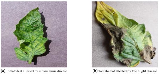
Figure 3. Examples of tomato leaves affected by diseases taken from the PlantVillage data-set ^[40].

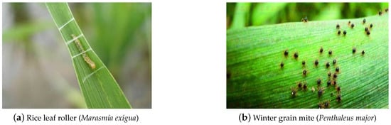
Figure 4. Examples of insect images taken from the IP102 data-set ^[41].

Tomato Powdery Mildew Disease (TPMD) is a different type of data-set because it is related to meteorological data. It offers statistics on powdery mildew disease susceptibility depending on a variety of weather-related variables such as humidity, wind speed, temperature, global radiation, and leaf wetness ^[45].

2.3. Field-Collected vs. Laboratory-Collected Data

ML models performance is influenced by the quality and type of input (image or other). Images acquired in a controlled laboratory environment and images acquired in the field can result in completely different processes and/or results. The difficulty for disease and pest classification is much higher for images acquired in the field than for images taken in a controlled environment.

Under a controlled laboratory environment, images typically contain a single leaf over a neutral artificial background ^[46]. The PantVillage data-set is an example of such situation ^[40]. It is possible to achieve great performance on these data-sets ^[1]. However, the creation of these types of data-sets is a time consuming and costly process.

When compared with images acquired in the laboratory, field images have much higher complexity, due to the presence of multiple leaves in the same image, presence of other plant parts, different shading, and lighting conditions, different ground textures, different backgrounds, etc. ^[42]. According to the studies in ^[42]^[47], training ML models using laboratory images provides poor outcomes when tested in the field, making them useless for the task. Training on field photographs and testing on laboratory photographs, on the other hand, produce reasonable outcomes ^[47]. The addition of field images in the training data has been shown to boost the results significantly, however testing on images from alternative data sources is advised ^[47]. PlantDoc demonstrates that cropping the leaves improves the accuracy of CNN architectures when dealing with in-field photos ^[42].

Table 1 shows the performance achieved on a few studies that analysed the impact of image acquisition conditions on the performance of disease classification models. In each table cell, “L” corresponds to lab images, “F” to field images and “L + F” for both types of images. In addition, the data-sets associated to the weights of the pre-trained models that were used for Transfer Learning are also shown.

Table 1. Performance comparison of field vs. laboratory data.

Study	Pretrained Weights	Training	Testing	Performance
^[47]	-	L	F	33.0% acc.
		F	L	65.0% acc.
		L + F	L + F	99.0% acc.
^[42]	ImageNet	L	F	15.0% acc.
	ImageNet + PlantVillage	F	F	30.0% acc.
	ImageNet + PlantVillage	F (cropped images)	F (cropped images)	70.0% acc.
^[1]	ImageNet	L	L	99.0%+ acc.

3. Data Pre-Processing

Pre-processing data before feeding it to the model is common in most ML-based applications. Images are typically pre-processed using computer vision techniques to remove noise, to enhance the image contrast, to extract the regions of interest, to extract image features, etc. In general, image pre-processing steps usually lead to better model outcomes. The most common data pre-processing techniques are covered in the following sub-sections.

3.1. Noise Reduction

Different types of filters, such as Gaussian and median filters, are used to reduce noise to obtain smoother images. These filters have an effect of blurring and removing non relevant details of an image, at the expense of potentially losing relevant textures or edges ^[48].

Erosion and dilatation are two morphological image operations that can be applied to binary or grey-scaled images. Erosion removes islands and tiny items, leaving only larger objects. In other words, it shrinks the foreground objects. On the other hand, dilation increases the visibility of items and fills in tiny gaps, adding pixels to the boundaries of objects in an image ^[49]. These operations reduce details and enhance regions of interest. These methods are helpful, for instance, for pest detection against a neutral background, such as images of traps with captured insects ^[6]^[50].

Images are usually stored in the RGB format, which is an additive color model of red, green, and blue components. Due to the high correlation between these color components, it is usually not suitable to perform color segmentation in the RGB color space. Therefore it is important to bear in mind that there are others color spaces such as HSV or L*a*b*. In HSV the color components are: hue (pure color), saturation (shade or amount of grey), and value (brightness). In the L*a*b* color space, L* is the luminance (brightness), a* is the value along the red-green axis, and b* is the value along the blue-yellow axis. In these color spaces, the brightness of a color is decoupled from its chromaticity, allowing the images to be processed with different lighting conditions ^[48]. This is significant in the context of agricultural images acquired in the fields, since they can have been shot under various lighting circumstances or at different times of the day.

Histogram equalization is a technique for adjusting contrast. In low contrast images, the range of intensity values is smaller than in high contrast images. Equalization of the histogram spreads out the intensity levels throughout values in a wider range. Contrast enhancement is not directly applied in the RGB color space, because it applies to brightness values. Thus, images have to be converted either to grey-scale or to a color space that contains a brightness component, such as the HSV or L*a*b* color spaces ^[48].

3.2. Image Segmentation

Image segmentation is the process of grouping pixels into regions of interest. In the context of crop disease identification, these regions of interest can be, for instance, diseased areas on the plant leaves, for assessing the severity of the infection by the amount of the infected area, or for background removal, since the removal of the background allows highlighting of the regions of interest for further analysis. An example of background removal is shown in Figure 5.

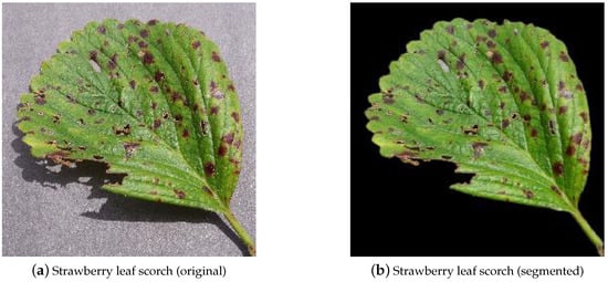
Figure 5. Example of background removal from the PlantVillage data-set ^[29].

Blob detection is a computer vision technique for getting regions of pixels that share common properties. The properties of these regions, such as color and brightness, differ greatly compared to their surroundings. This technique can be used, for instance, to detect and count insects in images ^[6]^[50].

The k-means clustering algorithm is a popular unsupervised ML algorithm that can be used for image segmentation. Pixels are grouped into clusters which have pixels with similar color and brightness values. This technique is helpful, for instance, to detect damaged regions on leaves ^[9]^[51]. Fuzzy c-means is a soft clustering technique where a pixel can be assigned to more than one group. This method was used by Sekulska-Nalewajko and Goclawski ^[52] and Zhou et al. ^[53] for plant disease classification.

Region growing is a region-based image segmentation technique used by Pang et al. in ^[54] to accurately define the image regions corresponding to the plant leaf parts affected by disease.

Intensity thresholding is a straightforward and simplified approach for image segmentation. According to the pixel value, that pixel is classified into a group (e.g., healthy or diseased). When using this technique, images are frequently converted to grey-scale first and then thresholded using a grey intensity value ^[55]. Figure 6 shows an example of an image converted to grey-scale.

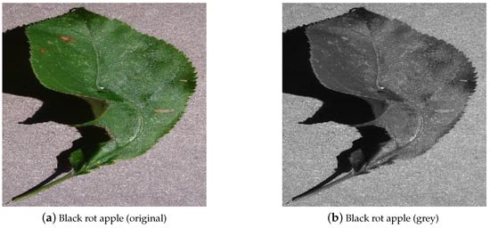
Figure 6. Example of an image converted to grey-scale from the PlantVillage data-set ^[29].

3.3. Feature Extraction

Feature extraction is a common step in the pre-processing of images for shallow ML models. Common image feature extraction algorithms include the Histogram of oriented Gradient (HoG), Speeded Up Robust Features (SURF) and Scale Invariant Feature Transform (SIFT) ^[41]^[56]. Different feature extractors obtain different features that can be more or less suitable for the specific problem at hand. HoG focuses on the structure and shape of the image objects, by detecting edges on images oriented according to different directions. The distribution of gradients according to these directions are used as features. SIFT finds scale and rotation invariant local features through the whole image, obtaining a set of image locations referred to as the image’s key-points. SURF is conceptually similar to SIFT, with the advantage of being much faster, which can be relevant for the implementation of real-time applications.

The distribution of image colors is represented by a color histogram. Since most diseases have symptoms that impact the color of the leaves, the histogram can also be used for distinguishing between healthy and unhealthy plants ^[56].

Some computer vision algorithms for feature extraction demand that pictures are converted to grey-scale, such as Haralick texture ^[57] or edge detection algorithms ^[58], etc. Haralick texture features are computed from a Grey Level Co-occurrence Matrix (GLCM), a matrix that counts the co-occurrence of neighboring grey-levels in the image. The GLCM acts as a counter for every combination of grey-level pairs in the image. Diseased and healthy leaves have different textures since a diseased leaf has a more irregular surface and a healthy leaf has a smoother one. These features allow differentiation of a healthy leaf from a diseased one.

Local Binary Pattern (LBP) ^[59] is another technique used for image texture features extraction robust to variations on lighting conditions. The LBP technique was used by Tan et al. in ^[60] for the extraction of information about diseases on tomato leaves.

Multi-spectral image data-sets can be exploited to create new data and improve the performance of models. For instance, in ^[18], originally, there were NIR pictures of the fields and from this data the authors created new images from spectral differences (between green and blue bands, and between NIR and green bands), band ratios and dimension reduction using principal component analysis. The authors also assess which type of data achieves best performance on the models.

3.4. Cropping and Resizing Images

Cropping and resizing images is used for decreasing the input image dimensions, to allow greater processing speed or to fit hardware requirements. It can also be used for creating more data to train the models, for example, from a low number of high resolution pictures, a much higher number of low resolution images can be retrieved ^[18].

3.5. Pre-Processing in Tabular Data

Tabular data consisting of weather records was commonly found in the literature. When gathering data records with varying dates and locations, these records can be integrated in two ways: cross-year, where models are validated over the years at the same location, and cross-location, where models are validated across the various locations for the same year. The average coefficient of determination (

r^{2}

) was found to be higher for cross-year models for all ML algorithms tested ^[7].

Common procedures in pre-processing are scaling/standardization of data and missing values processing ^[2]. Most algorithms require that there are no missing values in data and others, such as neural networks, can benefit from the normalization of feature values to improve training and reduce the effects of vanishing gradients ^[7].

Down sampling is a useful way to process data when there is a high number of records. In ^[31], measurements of leaf reflectance were done, from 760 to 2500 nm with a 1 nm interval. The 1740 wavelengths measurements were compressed into 174, and afterwards 10 wavelengths were selected using the stepwise method. From the regression analysis, results showed a coefficient of determination

r^{2} = 0.94

for these wavelengths and leaf severity. Experiments showed that fewer than those 10 wavelengths would worsen performance.

3.6. Pre-Processing in Deep Learning

Deep learning pre-processing does not focus on feature extraction since one of the most essential and beneficial properties of deep learning is its ability to generate features autonomously. For this reason, pre-processing is focused mainly on creating more images through data augmentation and resizing the input images to fit the models input parameters.

Some studies have compared the manual selection of features with deep learning. When it comes to categorizing insects in the field, manually selected features were not able to capture all of the relevant information about insect infestations or to handle the noise of real-world photos. Manually selected features were also not able to capture subtle differences between different insect species that share similar appearance ^[41]. For insect detection, deep learning techniques achieved higher accuracy and took less time to process since they efficiently select regions of interest ^[3]. In the work done by Brahimi et al. in ^[46], tomato disease classification using deep learning achieves higher accuracy, with values above 98%, but the accuracy of models using feature extractors is not very far behind, reaching values above 94%.

When comparing the use of original color pictures with images converted to grey-scale or background segmentation, deep learning models performed better in the original color pictures ^[1]. These findings are also confirmed in ^[61], where the performance of color vs. grey-scale pictures is compared. This supports the idea of deep learning not requiring extensive pre-processing of images. Nevertheless cropping images achieve better performance on field images classification, by increasing the region of interest and reducing the varying background ^[42].

Data augmentation is a process to artificially expand and increase the diversity of the training data-set. This process benefits the performance of the models, by introducing variability in the data and allowing a better generalization of the domain ^[62]. Some common transformations are rotation, cropping, scaling, and flipping.

Data cleaning is the process of assessing the quality of the data and to either modify or delete it. It is usually applied in studies that retrieve their data-set images from search engines in an automatic way, removing pictures that do not correspond to the intended labels or that do not comply with minimum resolution requirements ^[8]^[41].

Image resizing is usually performed to fit the input parameters of the models. Studies have compared the performance of the models with different input image sizes, and concluded that with larger images the models achieve higher accuracy but require more time for each training epoch ^[47] and more powerful hardware ^[50].

Table 2 shows the pre-processing techniques applied to deep learning classification models analysed herein. The ‘type’ column shows the data pre-processing technique used and the ‘info’ column contains additional details about it.

Table 2. Pre-processing when deep learning techniques were used.

Study	Type	Info
^[1]	Greyscale	-
	Background Segmentation	Masks
	Resize	256 × 256
^[8]	Data Augmentation	Affine, perspective, rotation
	Data Cleaning	-
	Resize	256 × 256
^[50]	Resize	52 × 52, 112 × 112, 224 × 224
^[41]	Data Cleaning	-
^[41]	Resize	224 × 224
^[3]	Data Augmentation	Crop, rotation, Gaussian noise, scale, flip
^[3]	Resize	600 × 1024, 300 × 300
^[46]	Resize	256 × 256
^[47]	Resize	256 × 256
^[61]	Greyscale	-
^[61]	Resize	60 × 60

From the table, it is noticeable that all analysed papers employing deep learning-based techniques used image resizing. It is also worth mentioning that the application of data augmentation was found in 25% of the depicted works, and the same goes for image color conversion to grey-scale and data cleaning.

4. Machine Learning Models

ML models enable researchers to get insight into data and existing correlations between various factors that influence occurrence of diseases and pests in crops. After data is processed and features are extracted, models can be used for classification, regression, among other goals. In classification, a new data sample is assigned a label according to the relations retrieved during the training process. In regression, a continuous output value is estimated from the input variables.

The following sub-sections contain a description about the ML models used, published work that have used them and the achieved performances. In addition, as a consequence of the conducted research, it was decided to include a sub-section about the use and potential of Transfer Learning (TF) in the research under consideration.

4.1. Support Vector Machine

SVM ^[63] is a model that creates a hyper-plane that separates two classes (can also be adapted and applied for multi-class problems). By maximizing the distance, or margin, between the nearest data points (support vectors) of each class to the hyper-plane, SVM chooses the optimum hyper-plane to segregate the data. SVM can also perform well in non-linear data by using the so called kernel trick technique. The SVM kernel is a function that transforms a low dimensional input space into a higher dimensional space that is linearly separable. For this reason, SVM can be very effective in high dimensional spaces. SVM can also be used for regression problems ^[7]^[18]^[64]. Furthermore SVM can also be used in a hybrid way as Bhatia et al. did in ^[65], by using SVM together with logistic regression algorithm to predict powdery mildew disease in tomato plant.

A syntheses of agricultural studies using SVM as the ML model can be observed in Table 3. The type of SVM used, as well as its kernel and result can be observed. Linear, polynomial, and RBF kernels seem to be most commonly used on SVM-based classification and regression algorithms applied to agriculture contexts.

Table 3. SVM performance.

Study	Classification/ Regression	Kernels
Study	Classification/ Regression	Type	Results
^[31]	Classification	Polynomial	90.0% acc.
^[31]	Classification	Radial Basis Function	97.4% acc.
^[7]	Regression	Not specified	SVM outperformed
^[18]	Regression	Linear	$r^{2}$ = 0.45
^[5]	Classification	Linear	90.0%+ acc.
^[9]	Classification	Radial Basis Function	90.5% acc.
		Quadratic	92.0% acc.
		Linear	91.0% acc.
		Multi-Layer Perceptron
		Polynomial
^[46]	Classification	Not specified	94.6% acc., 93.1% f1

SVM can achieve better performance than other ML techniques such as ANNs and conventional regression approaches in forecasting plant diseases ^[7].

4.2. Random Forest

Random Forest (RF) is a widely known ensemble built from decision trees trained on different subsets of the training data. Also, when deciding which variable to split on a node, RF considers a random set of variables and not the whole set of features. During classification, each tree votes and the class most agreed upon is returned. As each tree is trained on a subset of data and of features, the computation is fast. A high number of trees and the diversity of each of them makes them robust to noise and outliers. Some studies that have employed Random Forest (RF) are shown in Table 4.

Table 4. Performance of Random Forests.

Study	Classification/Regression	Number of Trees	Performance
^[18]	Regression	100	$r^{2}$ = 0.75
^[10]	Regression	200	$r^{2}$ = 0.75
^[56]	Classification	-	70.0% acc.
^[46]	Classification	-	95.5% acc., 94.2% f1

RFs can achieve greater accuracy with less number of samples when compared to other ML techniques ^[56].

4.3. Artificial Neural Networks

Artificial Neural Networks (ANN) are models inspired by biological brains. ANN consists of neurons distributed in input, hidden, and output layers and can have multiple hidden layers and multiple units in each layer. With more hidden layers, an ANN is able to learn complex relations from the hierarchical combination of multiple features, and thus create high-order features, Figure 7 shows an illustration of an ANN. Deep learning is associated with ANNs that contain a large amount of layers.

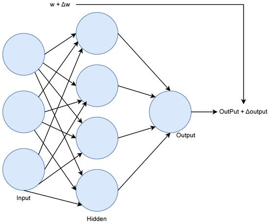
Figure 7. ANN example.

Learning occurs by a process called optimization, which is an iterative method for minimizing an error function, typically based the Gradient Descent algorithm. Instead of calculating the gradient from the entire data-set, the optimization process typically uses chunks of data records called batches. After the network processes the input, the output is compared to the expected output and the error is computed. The error is then propagated back through the network, one layer at a time, and the weights are updated according to the amount they contributed to the error. This updating process is called back-propagation. After all records in the data-set are processed once, a training epoch is completed. Training the network can require several epochs until desired results are achieved.

CNNs are a type of a deep learning network that commonly are applied on image classification tasks. In this type of network, the use of the so-called convolutional layers enables an hierarchical extraction of features, where simpler features such as edges are extracted in the first layers and more specific and complex features are extracted in deeper layers. The dimensionality of the input is decreased by the use of pooling layers. Fully connected neural networks are usually placed on top after the convolutional and pooling layers and act as classifiers using these high-level features.

Recurrent Neural Networks (RNN) are also a type of deep learning network, usually applied to time series data. RNNs extract features automatically from data and can capture temporal relationships. Because of the architecture of these networks, the gradients calculated to update the weights can become unstable, becoming too high (Exploding Gradient) or too low (Vanishing Gradient).

The recurrent layers can be structured in a wide variety of ways to produce distinct RNNs ^[66]. The LSTM cell was proposed by Hochreiter and Schmidhuber in ^[67]. Here, the remembering capacity for the standard recurrent cell was improved in order to deal with undesirable dependencies on the long-term.

Recently, Xiao et al. suggested in ^[2] that LSTM networks have specific advantages in processing time-dependent problems. LSTM networks can be used, for example, to retrieve relationships between meteorological data and pest occurrence in order to forecast future pest attacks.

In the context of agriculture, obtaining a large amount of annotated data for the training of ML-based algorithms can be a rather difficult task. Few-shot learning approaches have been trying to mitigate this problem by managing to learn with fewer data. The methods typically associated with this technique can be organized according to four groups ^[68]: data augmentation, metric learning, external memory, and parameter optimization. Yang et al. present a survey on the developments, application, and challenges of this approach.

When using ANN models, authors might use one of two methods. They either create their own model designs or adopt well-known architectures that have been shown to perform well in previous studies, particularly CNN architectures for image classification.

User-Defined Network Architectures

This sub-section presents studies where the authors defined their own neural network architectures.

In ^[18], Duarte-Carvajalino et al. built and compared the outcome of two different neural networks models. The first model was a Multi-Layer Perceptron (MLP) with 2 hidden layers, each having half the number of nodes of the previous layer. The authors used a learning rate of 0.01, the Adamax optimizer, batch normalization and dropout with probability of 0.2 in all layers, and ReLU as activation function. The other model was a CNN trained using the same hyperparameters used on the MLP. The CNN consists of two convolutional layers using 20 filter kernels of size 3 × 3, followed by a max pooling layer of size 2 × 2. The succeeding network layers are another two convolutional layers using 40 filter kernels of size 5 × 5 followed by a max pooling layer. After flattening, a dense layer is added before the output is computed. It was concluded that the CNN achieved better results than the MLP.

In ^[2], an LSTM network was used for processing time series data, i.e., winter and autumn data. The LSTM network consisted of two fully connected layers with five hidden units each. The results showed that the LSTM network achieved the best performance with 92% accuracy when compared to RF, SVM, and K-Nearest Neighbors (KNN). The Apriori algorithm ^[69] was applied for interpretability.

Disease prediction for different regions was also studied with the use of an ANN in ^[7]. In this case, the back-propagation neural network ^[70] and the generalized regression neural network ^[71] models were used.

A model suggested by Patil and Kumar in ^[72] attempted to identify the link between weather variables and the emergence of 4 types of rice diseases. In this work, the authors used an ANN to perform the detection, identification and prediction of the appearance of diseases in rice crops. The meteorological data-set referred to data between 1989 and 2019. The ANN consisted of 8 neurons in the input layer, 15 in the 2 hidden layers, and 5 in the output layer.

In ^[73], Sharma et al. performed a prediction of the potato late blight disease based on meteorological data only, using an ANN. In this case, data from 2011 and 2015 was used. Several tests with different network activation functions and data-set splits were done. It was concluded that the larger the data-set, the better was the performed prediction.

In addition, other algorithms relying on meteorological data and ANNs for performing predictions have been proposed. In ^[74], Dahikar and Rode present an ANN for predicting which crop will grow best in a certain area. The predictions were based on weather and soil data. Refs. ^[75]^[76] proposed ANN-based models for predicting crop yield.

Convolutional Neural Network Architectures

Image classification has achieved great results, with various model architectures being developed over the last 10 years. Most of these deep learning models were proposed in the context of the “Large Scale Visual Recognition Challenge” (ILSVRC). These models include well-known architectures such as AlexNet, GoogleNet, VGG, and ResNet, which have been widely used for image classification in different application domains.

Table 5 summarizes a set of studies that used pre-existing CNN architectures, depicting the architecture used in their work and the corresponding results.

Table 5. Performance of CNN architectures.

Study	Architecture	Results
^[1]	GoogleNet	99.3%
^[1]	AlexNet	99.3%
^[8]	CaffeNet	96.3%
^[50]	VGG16	98.0% validation, 81.0% in new apple orchard
^[41]	GoogleNet	43.5% acc., 32.7% f1
	FPN	54.9% mAP 0.5
	ResNet	49.4% acc., 40.1% f1
	VGGNet	48.2% acc., 38.7% f1
	AlexNet	41.8% acc., 34.1% f1
^[46]	GoogleNet	98.7% acc., 97.1% f1
^[46]	AlexNet	99.2% acc., 98.5% f1
^[47]	AlexNet	99.4% acc.
^[47]	VGG16	99.5% acc.
^[42]	VGG16	60.4% acc., 60.0% f1
	InceptionResNet V2	70.5% acc., 70.0% f1
	Inception V3	62.1% acc., 61.0% f1
^[61]	LeNet	98.6% acc., 98.6% f1

As can be observed from Table 5, several CNN architectures developed over the last decade have been successfully used, showing great potential for agriculture applications. From these, the use of older CNN architectures such as AlexNet (2012), VGG16 (2014), and GoogleNet (2014) were found on 44%, 33%, and 33% of the analysed papers, respectively.

4.4. Transfer Learning

TF makes use of already existing knowledge for some related task or domain in order and apply it to the problem under study. Models previously trained for image classification on large data-sets are usually used and adapted to the data-set under study. A common approach is to substitute the last network layers (i.e., the dense layers) of a pre-trained network, adapting it for a different classification task. The model is then trained but only the newly inserted layers are trainable—all network layers remain frozen during the training process. In extension of this approach, fine-tuning, is also commonly used. Besides training the newly inserted layers, fine-tuning allows the training of additional layers of the base model, typically the deeper convolutional layers of the network.

TF is usually done when the studied data-set is small, with insufficient samples for training a CNN model from scratch.

Table 6 synthesizes several deep learning-based studies where TF was applied. It presents details addressing: the data-set used for the base model training, the used TF method and the performance difference between using TF and training from scratch.

Table 6. TF analysis.

Study	Model	Dataset for Pretrain	Method	Performance Difference Compared to Training from Scratch
^[1]	AlexNet, GoogleNet	ImageNet	All layers trainable	~−2% acc.
^[8]	CaffeNet	ImageNet	Low learning rate for original layers (0.1), high for top layer (10)	~−0.50% acc.
^[41]	AlexNet, GoogleNet, VGGNet, ResNet	ImageNet	Fine tune	~−14.0% acc. in best model (ResNet)
^[3]	Faster RCNN (ResNet101, Inception V2, Inception ResNet V2)	COCO	Fine tune	No comparison
^[46]	AlexNet, GoogleNet	ImageNet	Fine tune	~−2%
^[42]	VGG16, Inception V3, Inception ResNet v2	ImageNet and/or PlantVillage	Fine tune	~−31.0% using ImageNet and PlantVillage

As can be observed from the table, the use of TF leads to lower performance when compared with training the full model from scratch. Nevertheless, there are many cases where such a difference is small, which means that TF can indeed be a useful possibility when the data-set is not sufficiently large.

References

Mohanty, S.P.; Hughes, D.P.; Salathé, M. Using deep learning for image-based plant disease detection. Front. Plant Sci. 2016, 7, 1419.
Xiao, Q.; Li, W.; Kai, Y.; Chen, P.; Zhang, J.; Wang, B. Occurrence prediction of pests and diseases in cotton on the basis of weather factors by long short term memory network. BMC Bioinform. 2019, 20, 688.
Gutierrez, A.; Ansuategi, A.; Susperregi, L.; Tubío, C.; Rankić, I.; Lenža, L. A benchmarking of learning strategies for pest detection and identification on tomato plants for autonomous scouting robots using internal databases. J. Sens. 2019, 2019, 5219471.
Choudhuri, K.B.R.; Mangrulkar, R.S. Data Acquisition and Preparation for Artificial Intelligence and Machine Learning Applications. In Design of Intelligent Applications Using Machine Learning and Deep Learning Techniques; Chapman and Hall/CRC: Boca Raton, FL, USA, 2021; pp. 1–11.
Raza, S.E.A.; Prince, G.; Clarkson, J.P.; Rajpoot, N.M. Automatic detection of diseased tomato plants using thermal and stereo visible light images. PLoS ONE 2015, 10, e0123262.
Rustia, D.J.A.; Lin, T.T. An IoT-based wireless imaging and sensor node system for remote greenhouse pest monitoring. Chem. Eng. Trans. 2017, 58, 601–606.
Kaundal, R.; Kapoor, A.S.; Raghava, G.P. Machine learning techniques in disease forecasting: A case study on rice blast prediction. BMC Bioinform. 2006, 7, 485.
Sladojevic, S.; Arsenovic, M.; Anderla, A.; Culibrk, D.; Stefanovic, D. Deep neural networks based recognition of plant diseases by leaf image classification. Comput. Intell. Neurosci. 2016, 2016, 3289801.
Mokhtar, U.; Ali, M.A.; Hassanien, A.E.; Hefny, H. Identifying two of tomatoes leaf viruses using support vector machine. In Information Systems Design and Intelligent Applications; Springer: Berlin/Heidelberg, Germany, 2015; pp. 771–782.
Skawsang, S.; Nagai, M.; K. Tripathi, N.; Soni, P. Predicting rice pest population occurrence with satellite-derived crop phenology, ground meteorological observation, and machine learning: A case study for the Central Plain of Thailand. Appl. Sci. 2019, 9, 4846.
Significant Remote Sensing Vegetation Indices a Review of Developments and Applications. Available online: https://www.hindawi.com/journals/JS/2017/1353691/ (accessed on 11 January 2022).
Abdulridha, J.; Ampatzidis, Y.; Kakarla, S.C.; Roberts, P. Detection of target spot and bacterial spot diseases in tomato using UAV-based and benchtop-based hyperspectral imaging techniques. Precis. Agric. 2020, 21, 955–978.
Earth Observing System Vegetation Indices to Drive Digital Agri Solutions. Available online: https://eos.com/blog/vegetation-indices/ (accessed on 11 January 2022).
Evangelides, C.; Nobajas, A. Red-Edge Normalised Difference Vegetation Index (NDVI705) from Sentinel-2 imagery to assess post-fire regeneration. Remote Sens. Appl. Soc. Environ. 2020, 17, 100283.
Albetis, J.; Duthoit, S.; Guttler, F.; Jacquin, A.; Goulard, M.; Poilvé, H.; Féret, J.B.; Dedieu, G. Detection of Flavescence dorée grapevine disease using unmanned aerial vehicle (UAV) multispectral imagery. Remote Sens. 2017, 9, 308.
Chandel, A.K.; Khot, L.R.; Sallato, B. Apple powdery mildew infestation detection and mapping using high-resolution visible and multispectral aerial imaging technique. Sci. Hortic. 2021, 287, 110228.
Wang, F.M.; Huang, J.F.; Tang, Y.L.; Wang, X.Z. New vegetation index and its application in estimating leaf area index of rice. Rice Sci. 2007, 14, 195–203.
Duarte-Carvajalino, J.M.; Alzate, D.F.; Ramirez, A.A.; Santa-Sepulveda, J.D.; Fajardo-Rojas, A.E.; Soto-Suárez, M. Evaluating late blight severity in potato crops using unmanned aerial vehicles and machine learning algorithms. Remote Sens. 2018, 10, 1513.
Kim, S.; Lee, M.; Shin, C. IoT-based strawberry disease prediction system for smart farming. Sensors 2018, 18, 4051.
Yin, X.; Kropff, M.J.; McLaren, G.; Visperas, R.M. A nonlinear model for crop development as a function of temperature. Agric. For. Meteorol. 1995, 77, 1–16.
Henderson, D.; Williams, C.J.; Miller, J.S. Forecasting late blight in potato crops of southern Idaho using logistic regression analysis. Plant Dis. 2007, 91, 951–956.
Lasso, E.; Corrales, D.C.; Avelino, J.; de Melo Virginio Filho, E.; Corrales, J.C. Discovering weather periods and crop properties favorable for coffee rust incidence from feature selection approaches. Comput. Electron. Agric. 2020, 176, 105640.
Small, I.M.; Joseph, L.; Fry, W.E. Development and implementation of the BlightPro decision support system for potato and tomato late blight management. Comput. Electron. Agric. 2015, 115, 57–65.
Ghaffari, R.; Zhang, F.; Iliescu, D.; Hines, E.; Leeson, M.; Napier, R.; Clarkson, J. Early detection of diseases in tomato crops: An electronic nose and intelligent systems approach. In Proceedings of the 2010 International Joint Conference on Neural Networks (IJCNN), Barcelona, Spain, 18–23 July 2010; pp. 1–6.
Holopainen, J.K. Multiple functions of inducible plant volatiles. Trends Plant Sci. 2004, 9, 529–533.
Diepeveen, D.; Armstrong, L.; Vagh, Y. Identifying key crop performance traits using data mining. In Proceedings of the IAALD-AFITA-WCCA Congress 2008 (World Conference on Agricultural Information and IT), Tokyo, Japan, 25–27 August 2008.
Patil, N.N.; Saiyyad, M.A.M. Machine learning technique for crop recommendation in agriculture sector. Int. J. Eng. Adv. Technol. 2019, 9, 1359–1363.
Rosenzweig, C.; Iglesius, A.; Yang, X.B.; Epstein, P.R.; Chivian, E. Climate Change and Extreme Weather Events-Implications for Food Production, Plant Diseases, and Pests; NASA Publications: Nebraska, NU, USA, 2001.
PlantVillage Tomato | Diseases and Pests, Description, Uses, Propagation. Available online: https://plantvillage.psu.edu/topics/tomato/infos (accessed on 11 January 2022).
Deutsch, C.A.; Tewksbury, J.J.; Tigchelaar, M.; Battisti, D.S.; Merrill, S.C.; Huey, R.B.; Naylor, R.L. Increase in crop losses to insect pests in a warming climate. Science 2018, 361, 916–919.
Dake, W.; Chengwei, M. The support vector machine (SVM) based near-infrared spectrum recognition of leaves infected by the leafminers. In Proceedings of the First International Conference on Innovative Computing, Information and Control-Volume I (ICICIC’06), Beijing, China, 30 August–1 September 2006; Volume 3, pp. 448–451.
Measuring Vegetation NDVI and EVI. Available online: https://earthobservatory.nasa.gov/features/MeasuringVegetation/measuring_vegetation_2.php (accessed on 11 January 2022).
Herbert, D.A.; Mack, T.; Reed, R.B.; Getz, R. Degree-Day Maps for Management of Soybean Insect Pests in Alabama; Auburn University: Auburn, AL, USA, 1988.
Research Models: Insects, Mites, Diseases, Plants, and Beneficials-from UC IPM. Available online: http://ipm.ucanr.edu/MODELS/models_scientific.html (accessed on 10 July 2014).
Entomology, L.O.E. Temperature-Dependent Development of Greenhouse Whitefly and Its Parasite Encarsia formosa. Environ. Entomol. 1982, 11, 483–485.
Miller, P.; Lanier, W.; Brandt, S. Using Growing Degree Days to Predict Plant Stages; Ag/Extension Communications Coordinator, Communications Services, Montana State University-Bozeman: Bozeman, MO, USA, 2001; Volume 59717, pp. 994–2721.
Calculating Degree Days. Available online: https://www.degreedays.net/calculation (accessed on 26 July 2022).
Tomato Diseases and Disorders|Home and Garden Information Center. Available online: https://hgic.clemson.edu/factsheet/tomato-diseases-disorders/ (accessed on 26 May 2021).
Seager, S.; Turner, E.L.; Schafer, J.; Ford, E.B. Vegetation’s red edge: A possible spectroscopic biosignature of extraterrestrial plants. Astrobiology 2005, 5, 372–390.
Hughes, D.; Salathé, M. An open access repository of images on plant health to enable the development of mobile disease diagnostics. arXiv 2015, arXiv:1511.08060.
Wu, X.; Zhan, C.; Lai, Y.K.; Cheng, M.M.; Yang, J. Ip102: A large-scale benchmark dataset for insect pest recognition. In Proceedings of the IEEE/CVF Conference on Computer Vision and Pattern Recognition, Long Beach, CA, USA, 15–20 June 2019; pp. 8787–8796.
Singh, D.; Jain, N.; Jain, P.; Kayal, P.; Kumawat, S.; Batra, N. PlantDoc: A dataset for visual plant disease detection. In Proceedings of the 7th ACM IKDD CoDS and 25th COMAD, Hyderabad, India, 5–7 January 2020; pp. 249–253.
Wu, S.G.; Bao, F.S.; Xu, E.Y.; Wang, Y.X.; Chang, Y.F.; Xiang, Q.L. A leaf recognition algorithm for plant classification using probabilistic neural network. In Proceedings of the 2007 IEEE International Symposium on Signal Processing and Information Technology, Giza, Egypt, 15–18 December 2007; pp. 11–16.
Lee, S.H.; Chan, C.S.; Mayo, S.J.; Remagnino, P. How deep learning extracts and learns leaf features for plant classification. Pattern Recognit. 2017, 71, 1–13.
Bakeer, A.; Abdel-Latef, M.; Afifi, M.; Barakat, M. Validation of tomato powdery mildew forecasting model using meteorological data in Egypt. Int. J. Agric. Sci. 2013, 5, 372.
Brahimi, M.; Boukhalfa, K.; Moussaoui, A. Deep learning for tomato diseases: Classification and symptoms visualization. Appl. Artif. Intell. 2017, 31, 299–315.
Ferentinos, K.P. Deep learning models for plant disease detection and diagnosis. Comput. Electron. Agric. 2018, 145, 311–318.
Garcia-Lamont, F.; Cervantes, J.; López, A.; Rodriguez, L. Segmentation of images by color features: A survey. Neurocomputing 2018, 292, 1–27.
Types of Morphological Operations MATLAB and Simulink. Available online: https://www.mathworks.com/help/images/morphological-dilation-and-erosion.html. (accessed on 11 January 2022).
Albanese, A.; d’Acunto, D.; Brunelli, D. Pest detection for precision agriculture based on iot machine learning. In International Conference on Applications in Electronics Pervading Industry, Environment and Society; Springer: Berlin/Heidelberg, Germany, 2019; pp. 65–72.
Sannakki, S.S.; Rajpurohit, V.S.; Nargund, V.; Kumar, A.; Yallur, P.S. Leaf disease grading by machine vision and fuzzy logic. Int. J. 2011, 2, 1709–1716.
Sekulska-Nalewajko, J.; Goclawski, J. A semi-automatic method for the discrimination of diseased regions in detached leaf images using fuzzy c-means clustering. In Proceedings of the Perspective Technologies and Methods in MEMS Design, Polyana, Ukraine, 1–14 May 2011; pp. 172–175.
Zhou, Z.; Zang, Y.; Li, Y.; Zhang, Y.; Wang, P.; Luo, X. Rice plant-hopper infestation detection and classification algorithms based on fractal dimension values and fuzzy C-means. Math. Comput. Model. 2013, 58, 701–709.
Pang, J.; Bai, Z.y.; Lai, J.c.; Li, S.k. Automatic segmentation of crop leaf spot disease images by integrating local threshold and seeded region growing. In Proceedings of the 2011 International Conference on Image Analysis and Signal Processing, Wuhan, China, 21–23 October 2011; pp. 590–594.
Patil, S.B.; Bodhe, S.K. Leaf disease severity measurement using image processing. Int. J. Eng. Technol. 2011, 3, 297–301.
Ramesh, S.; Hebbar, R.; Niveditha, M.; Pooja, R.; Shashank, N.; Vinod, P. Plant disease detection using machine learning. In Proceedings of the 2018 International Conference on Design Innovations for 3Cs Compute Communicate Control (ICDI3C), Bangalore, India, 25–28 April 2018; pp. 41–45.
Haralick, R.M.; Shanmugam, K.; Dinstein, I.H. Textural features for image classification. IEEE Trans. Syst. Man Cybern. 1973, SMC-3, 610–621.
Heath, M.D.; Sarkar, S.; Sanocki, T.; Bowyer, K.W. A robust visual method for assessing the relative performance of edge-detection algorithms. IEEE Trans. Pattern Anal. Mach. Intell. 1997, 19, 1338–1359.
Ojala, T.; Pietikainen, M.; Harwood, D. Performance evaluation of texture measures with classification based on Kullback discrimination of distributions. In Proceedings of the 12th International Conference on Pattern Recognition, Jerusalem, Israel, 9–13 October 1994; Volume 1, pp. 582–585.
Tan, L.; Lu, J.; Jiang, H. Tomato Leaf Diseases Classification Based on Leaf Images: A Comparison between Classical Machine Learning and Deep Learning Methods. AgriEngineering 2021, 3, 542–558.
Amara, J.; Bouaziz, B.; Algergawy, A. A deep learning-based approach for banana leaf diseases classification. In Datenbanksysteme für Business, Technologie und Web (BTW 2017)-Workshopband; Gesellschaft für Informatik e.V.: Bonn, Germany, 2017.
Kamilaris, A.; Prenafeta-Boldú, F.X. Deep learning in agriculture: A survey. Comput. Electron. Agric. 2018, 147, 70–90.
Suthaharan, S. Support vector machine. In Machine Learning Models and Algorithms for Big Data Classification; Springer: Berlin/Heidelberg, Germany, 2016; pp. 207–235.
Gu, Y.; Yoo, S.; Park, C.; Kim, Y.; Park, S.; Kim, J.; Lim, J. BLITE-SVR: New forecasting model for late blight on potato using support-vector regression. Comput. Electron. Agric. 2016, 130, 169–176.
Bhatia, A.; Chug, A.; Singh, A.P. Hybrid SVM-LR classifier for powdery mildew disease prediction in tomato plant. In Proceedings of the 2020 7th International Conference on Signal Processing and Integrated Networks (SPIN), Noida, India, 27–28 February 2020; pp. 218–223.
Yu, Y.; Si, X.; Hu, C.; Zhang, J. A review of recurrent neural networks: LSTM cells and network architectures. Neural Comput. 2019, 31, 1235–1270.
Hochreiter, S.; Schmidhuber, J. Long short-term memory. Neural Comput. 1997, 9, 1735–1780.
Yang, J.; Guo, X.; Li, Y.; Marinello, F.; Ercisli, S.; Zhang, Z. A survey of few-shot learning in smart agriculture: Developments, applications, and challenges. Plant Methods 2022, 18, 28.
Agrawal, R.; Srikant, R. Fast algorithms for mining association rules. In Proceedings of the 20th International Conference on Very Large Data Bases, VLDB, Santiago, Chile, 12–15 September 1994; Volume 1215, pp. 487–499.
Buscema, M. Back propagation neural networks. Subst. Use Misuse 1998, 33, 233–270.
Specht, D.F. A general regression neural network. IEEE Trans. Neural Netw. 1991, 2, 568–576.
Patil, R.R.; Kumar, S. Predicting rice diseases across diverse agro-meteorological conditions using an artificial intelligence approach. PeerJ Comput. Sci. 2021, 7, e687.
Sharma, P.; Singh, B.; Singh, R. Prediction of potato late blight disease based upon weather parameters using artificial neural network approach. In Proceedings of the 2018 9th International Conference on Computing, Communication and Networking Technologies (ICCCNT), Bengaluru, India, 10–12 July 2018; pp. 1–13.
Dahikar, S.S.; Rode, S.V. Agricultural crop yield prediction using artificial neural network approach. Int. J. Innov. Res. Electr. Electron. Instrum. Control Eng. 2014, 2, 683–686.
Trenz, O.; Št’astnỳ, J.; Konečnỳ, V. Agricultural data prediction by means of neural network. Agric. Econ. 2011, 57, 356–361.
Ranjeet, T.; Armstrong, L. An Artificial Neural Network for Predicting Crops Yield in Nepal. In Proceedings of the Asian Federation for Information Technology in Agriculture, Perth, Australia, 29 September–2 October 2014.

© Text is available under the terms and conditions of the Creative Commons Attribution (CC BY) license; additional terms may apply. By using this site, you agree to the Terms and Conditions and Privacy Policy.

Upload a video for this entry

Information

Subjects: Agricultural Engineering; Automation & Control Systems; Computer Science, Artificial Intelligence

Contributors MDPI registered users' name will be linked to their SciProfiles pages. To register with us, please refer to https://encyclopedia.pub/register :

Tiago Domingues

Tomás Brandão

João C. Ferreira

View Times: 594

Update Date: 16 Sep 2022

Table of Contents

Video Upload Options

Confirm