Your browser does not fully support modern features. Please upgrade for a smoother experience.
Submitted Successfully!
 +1 credit
Thank you for your contribution! You can also upload a video entry or images related to this topic.
For video creation, please contact our Academic Video Service.
| Version | Summary | Created by | Modification | Content Size | Created at | Operation |
|---|---|---|---|---|---|---|
| 1 | Qi Zhang | -- | 1730 | 2022-08-16 14:41:55 | | | |
| 2 | Qi Zhang | + 1881 word(s) | 3611 | 2022-08-17 05:51:04 | | | | |
| 3 | Catherine Yang | Meta information modification | 3611 | 2022-08-17 06:02:34 | | |
Video Upload Options
We provide professional Academic Video Service to translate complex research into visually appealing presentations. Would you like to try it?
Cite
If you have any further questions, please contact Encyclopedia Editorial Office.
Zhang, Q. Exploring Trend of Commodity Prices. Encyclopedia. Available online: https://encyclopedia.pub/entry/26199 (accessed on 24 July 2026).
Zhang Q. Exploring Trend of Commodity Prices. Encyclopedia. Available at: https://encyclopedia.pub/entry/26199. Accessed July 24, 2026.
Zhang, Qi. "Exploring Trend of Commodity Prices" Encyclopedia, https://encyclopedia.pub/entry/26199 (accessed July 24, 2026).
Zhang, Q. (2022, August 16). Exploring Trend of Commodity Prices. In Encyclopedia. https://encyclopedia.pub/entry/26199
Zhang, Qi. "Exploring Trend of Commodity Prices." Encyclopedia. Web. 16 August, 2022.
Copy Citation
As the supply of commodities forms essential lifelines for modern society, commodity price fluctuations can significantly impact the operation and sustainable development of macroeconomics, production activities, and people’s security and well-being. The commodity trading market also plays a pivotal role in the competition of the international industrial chain and the sustainable development of the industry.
commodity prices
bibliometrics
co-citation
cluster analysis
1. Introduction
Commodities, essential lifelines for modern society, include almost all primary material commodities used for production and consumption, such as energy, minerals, and agricultural products. It is important to understand the driving factors for the fluctuations of commodity prices and the impact of commodity price changes on the macroeconomy [1]. In consumer and producer countries, a large part of income and welfare depends on the prices of these goods [2]. Commodity markets occasionally exhibit widespread mass booms and busts. These events affect the ability of the poor and those countries in the developing world to purchase basic necessities, such as food and energy, creating trade imbalance, and in some cases, political turmoil. The effect of the “boom and bust” of commodity prices resonates with ordinary people because trade imbalances and currency shocks that can then arise affect social welfare [3], the operation of the national economy, and enterprise production in a way that not all price surges do. Therefore, commodities price fluctuation has received attention from all quarters.
In addition, commodity prices are more volatile than others [4]. With the gradually deepening financialization of the commodity market, this greater fluctuation is obvious and is well known to be extremely susceptible to large-scale emergencies, creating rapid fluctuation. Starting from decade lows in the late 1990s, commodity prices continued to rise for the next 10 years, and reached their peak in June 2008. After the financial crisis, it was pushed to a record high by many countries’ economic stimulus. The price until 2011 was twice as much as that in 1988. From the second half of 2006 to the first half of 2008, driven by various factors, the prices of agricultural products on a global scale rose, triggering a round of food crises that seriously impacted the welfare of the poor worldwide. Due to the wide effects of COVID-19, the prices of metal products, such as steel and copper, fell sharply and then increased rapidly in 2020, posing a serious threat to the production and survival of downstream small- and medium-sized enterprises. In the long run, the trend of increasing volatility in commodity prices can be difficult to reverse, creating the necessity to pay more attention to the field of forecasting international commodity prices.
More importantly, the volatility of commodity prices has an important impact on the sustainable development of a country. Take energy as an example. Among the Sustainable Development Goals, SDG7 is the Sustainable Development Goal of Energy, which is to ensure that everyone has access to affordable, reliable, and sustainable modern energy. However, energy prices affect the stability and sustainable development of most countries, especially poor countries, where access to energy is limited; in addition, some populations have no access to energy at all, which goes against the goals of SDG7 [5]. On the other hand, sharp fluctuations in energy prices have had a significant impact, with rapid price declines not conducive to energy exporting countries; however, sharp price increases are unfavorable for energy importing countries, and exporting countries are affected by energy price vulnerability [6]. If the general trend of energy prices cannot be well grasped and a safe energy guarantee mechanism cannot be established, it will bring challenges to the sustainable development of the country [7][8]. Likewise, food sustainability is one of the main concepts for achieving global sustainable development [9]. SDG2 means ending hunger, achieving food security, improving nutrition, and promoting sustainable agriculture. High food prices will limit people’s ability to obtain food [10], which is fundamentally detrimental to the long-term development of the country.
Having a better understanding of the research history and development path of commodity prices, and grasping the current research hotspots and future development trends, are of theoretical and practical significance. In particular, it can help companies to prevent future business risks, help companies to take effective measures to hedge the cost risks caused by drastic price changes, and increase the expectations for future sustainable development. However, current research reviews in this field mainly use qualitative analysis methods, relying on an author’s subjective framework to sort out research themes and content [11], or only focusing on one specified commodity. For example, Chiroma et al. [12] reviewed the application of existing computer intelligence algorithms in crude oil price prediction, and analyzed the advantages and limitations of the research. Ederington et al. [13] reviewed the existing research on the relationship between crude oil prices and petroleum product prices, and summarized the causal and asymmetric relationship between the two. Abdallah et al. [14] used food safety, price fluctuations, and price transmission as keywords to quantitatively analyze literature on food safety and food prices; this revealed the current research hotspots and status quo.
2. Statistical Analysis of Commodity Prices
This section may be divided into subheadings. It should provide a concise and precise description of the experimental results, their interpretation, as well as the experimental conclusions that can be drawn.
2.1. Research on the Overall Growth Trend
The degree of academic attention to a certain field can be reflected in the number of publications and citations. It can be seen from Figure 1 that the literature on commodity prices has gradually increased since 2000, and has shown an explosive growth trend after 2008, reaching 221 in 2019. From 1990 to 2019, the number of documents has doubled a hundredfold in 30 years. This is in line with the actual situation. The 2008 financial crisis caused violent fluctuations in commodity prices and severely impacted economic operations. Since then, more scholars have devoted themselves to research in this field.
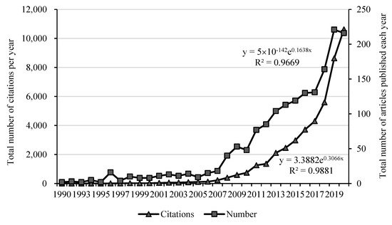
Figure 1. The number of published documents in each year (1990–2020).
Figure 1 also reflects the changing trend of the number of citations in the field of commodity prices in the past 30 years. The number of citations grew from 5 in 1990 to 10,624 in 2020. The most cited article is Kilian’s article published on AER in 2009. This groundbreaking research decomposed the actual price of crude oil into three parts: crude oil supply shocks, shocks to the global industrial commodity demand, and demand shocks specific to the crude oil market; it discussed the reasons for major oil price shocks since 1975. As of 2020, this article has been cited 1409 times, becoming a foundational work in the field of commodity prices.
For the quantitative work, our method was: apply exponential fitting to the number of articles published each year and the number of citations. The R-squares of the curves are 0.967 and 0.988, respectively, indicating that the number of research documents and citations in the field of commodity prices has exponentially increased; this reflects the high degree of concern of the academic community on commodity prices in recent years.
2.2. Publication Sources
Figure 2 shows the main research areas of commodity prices and their proportions. The research direction is given by the Web of Science database. Since the research content of a document may involve multiple fields, the proportions of each field add up to more than 100%. It can be seen that the research is mainly concentrated on economics and energy, with a small proportion of research focusing on finance.
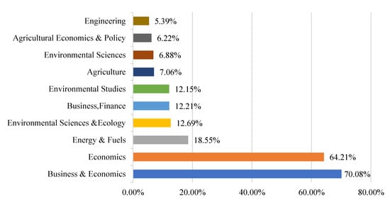
Figure 2. Main research areas and proportions.
Paying attention to publications of frequently cited literature can clarify the degree of academic attention to the field of commodity prices. Table 1 shows some highly cited journals and their impact factors in the past five years. Among them, Energy Economics, Journal of Econometrics, Econometrica, and American Economic Review are highly cited. They are the top publications in the fields of energy, econometrics, and economics. It shows that in addition to relevant professional knowledge, research on commodity prices also involves using a large number of econometric models. From the perspective of the volume of publications, the literature in this field is mostly concentrated on Energy Economics, Energy Policy, and Energy, and the impact factors of these journals are all above 6; this indicates that there has been a batch of high-quality articles affecting economic operation and resource management in the field of commodity price research.
Table 1. Statistics of highly cited articles published in journals.
| Citations | Number of Articles Published | Journal | 5 Year Impact Factor |
|---|---|---|---|
| 1051 | 269 | Energy Economics | 7.571 |
| 687 | 79 | Energy Policy | 6.581 |
| 324 | 54 | Energy | 6.845 |
| 466 | 44 | Economic Modelling | 3.412 |
| 433 | 41 | Energy Journal | 2.786 |
| 333 | 38 | Applied Economics | 1.88 |
| 227 | 38 | Resources Policy | 5.654 |
| 299 | 31 | Applied Energy | 9.953 |
| 119 | 30 | Applied Economics Letters | 1.2 |
| 207 | 27 | American Journal of Agricultural Economics | 4.461 |
2.3. Research Countries
Figure 3 shows the cooperation network in the country where the first author of the article is located. According to Figure 3, the United States, China, Australia, and France are at the center of the network, forming a relatively close cooperative relationship, and each has cooperation with many other countries. Judging from the average year of publication, the United States, Canada, and other countries started research in this area earlier. While China started late, Chinese authors quickly occupied the sub-center position of this network. Figure 4 summarizes the number of publications in the country of the first author. The United States (385) and China (341) have the largest number of publications. The sum of the number of articles from the two countries accounts for more than one-third of the total publications, followed by Australia (119), England (117), and France (104). The total number of articles by researchers in these five countries accounts for more than one-half of the total.
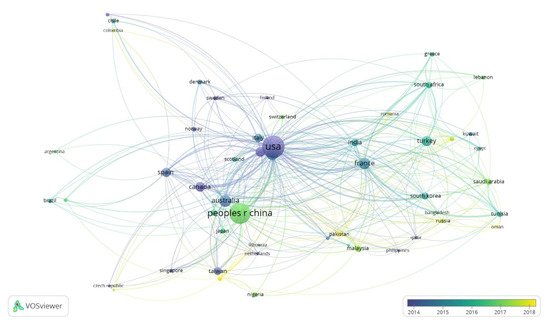
Figure 3. Cooperation network between countries.
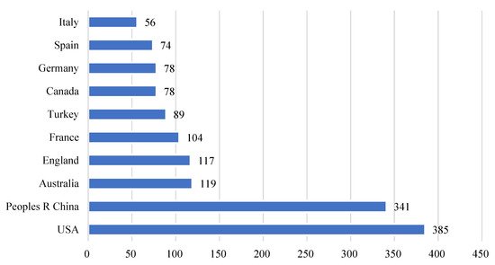
Figure 4. Distribution of research regions.
Next, we focus on the research object of the literature. Extract the names of countries or organizations from the topics, and make statistics in groups of five years to obtain the histogram shown in Figure 5. It can be seen that before the 21st century, scholars paid more attention to the situation in the United States, Gulf Cooperation Council countries, and Britain. After entering the 21st century, scholars’ research enthusiasm for the United States has not diminished. However, they no longer focus on the United Kingdom, but on the overall situation of EU countries. Since 2006, the number of publications in this field has increased sharply (Figure 1); emerging economies such as China and India have entered the research scope of scholars, especially China, which has become the largest research object in this field since 2011. In addition, after 2006, the diversity of research objects has increased, rather than focusing on just a few countries. At the same time, there are also many pieces of literature studying the situation of a group or groups of similar countries, such as oil importing countries, oil exporting countries, emerging economies, etc., or countries in the same region, such as the Middle East, Asia, South Africa, etc.
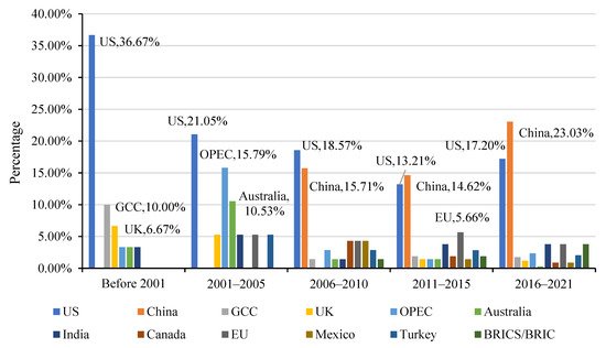
Figure 5. Distribution of the research object.
3. Co-Citation Analysis of Commodity Prices
3.1. Cluster Analysis of Co-Cited Articles
If two articles appear together in the reference list of the third citing document, these two references form a co-citation relationship. If the two documents are cited by n documents together, the number of co-citations is n times. According to co-citation analysis, the degree of correlation between documents can be measured, and the collection of documents can be classified according to the degree of correlation, after which a cluster analysis network diagram of professional papers in that discipline can be generated. In Figure 8, showing the co-citation network of sample articles, node size in the graph indicates the frequency of citations. The higher the frequency of citations, the larger the nodes. The connection between two nodes designates these two documents have been cited together. Indicating a change in the research direction, the color of the infographic changed from dark to light over the 1990 to 2020 period, and the research focus expanded from an agricultural commodity price and oil price dynamic to an oil price prediction and financialization.
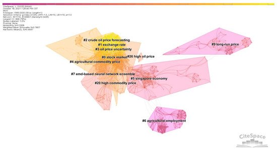
Figure 8. Clusters of co-cited articles.
In Table 4, which depicts a summary of each cluster’s details, cluster size represents the number of articles it includes. Silhouette is a parameter proposed by Kaufman and Rousseeuw in 1990 to evaluate the effect of clustering through network homogeneity [15]. The Silhouette value lies between 0–1, and the closer it is to 1, the higher the homogeneity of the network and the higher the credibility of clustering. The publication year is the average publication time of articles in this cluster. According to Table 4, the largest clusters are Cluster #0, #1, #2, #3, and #4. Their articles focus on the exploration of the correlation between commodity prices and the stock market, the exchange rate, oil price uncertainty, and crude oil price forecasting. In addition, most clusters’ Silhouette values are above 0.7, indicating that these clusters are highly homogeneous and highly reliable.
Table 4. Citation clustering network.
| Cluster ID | Cluster Label | Cluster Size | Silhouette | Year (Average) |
|---|---|---|---|---|
| #0 | stock market | 209 | 0.656 | 2006 |
| #1 | exchange rate | 141 | 0.698 | 2013 |
| #2 | crude oil price forecasting | 126 | 0.729 | 2012 |
| #3 | oil price uncertainty | 103 | 0.749 | 2014 |
| #4 | agricultural commodity price | 76 | 0.854 | 2009 |
| #5 | Singapore economy | 70 | 0.954 | 1996 |
| #6 | agricultural employment | 47 | 0.995 | 1991 |
| #7 | EMD-based neural network ensemble | 47 | 0.969 | 2001 |
| #9 | long-run price | 38 | 1 | 1993 |
| #20 | high commodity price | 7 | 0.996 | 2008 |
| #26 | high oil price | 4 | 0.996 | 2003 |
The citation network and cluster analysis show that the research hotspots of commodity prices focus on influencing factors, impacts on macroeconomy, price forecasts, and commodity financialization; moreover, these hotspots form a research network centered on oil prices. The detailed discussion is shown in Table 5:
- (1)
-
Influencing factors of commodity prices (Cluster #1, #9, #20, #26)
The influencing factors of commodity price fluctuations have been widely focused on by many scholars. The contradiction between supply–demand and inventory change are generally considered the basic factors affecting international commodity price fluctuations. Since the operation of the global economy is fundamental to commodity supply and demand, but financial markets can have a spillover effect into the commodity market, the coordinated change of commodity prices becomes a goalpost for planners. Speculative factors have pushed up the prices of major commodities in the past, making the strong demand from emerging economies another reason for the overall rise in commodity prices. Factors including natural disasters, cyclical changes in production, and policy adjustments also considerably impact commodity prices. Differences in national economic systems also lead to differences in commodity prices between countries. The economic system affects the speed and strength of the transmission of international commodity prices to domestic commodity prices, and ultimately reflects in domestic prices.
A substantial increase or decrease in commodity prices frequently results from a combination of multiple factors. Hamilton [16] studied some factors leading to changes in crude oil prices, including supply and demand, commodity speculation, monopolistic oligarchs, and resource depletion. Mueller et al. [17], analyzing the reasons why food prices doubled in the world from March 2007 to March 2008, found multiple factors, including greater energy and fertilizer costs, increased financial speculation in commodity markets, export restrictions, dollar depreciation, biofuel production increase, poor harvests, reduced world food reserves, increased foreign exchange reserves, and the continuing increase in world population and expectations of affluence.
Academic circles have continuously analyzed the factors affecting commodity price fluctuations. Ranging from the basics of supply and demand to the impact of financial speculation and analysis of interruptive events, and from linear to nonlinear, the research in these directions continues to deepen comprehensively [18][19][20][21][22][23][24][25].
- (2)
-
The impact of commodity price fluctuations on macro economy (Cluster #3, #4, #5, #6)
The impact of commodity price fluctuations on the macroeconomy is another noteworthy research direction that has developed to a great extent.
Building on the foundational work of Hamilton [26] four decades ago, scholars have segued to study the oil price–economic growth relationship [27][28][29][30] or taken up nonlinear perspective considerations [31][32][33]. Important in international trade, the relationship between commodity prices and exchange rates has also received key attention. Chen [34] used monthly panel data from G7 countries to study the long-term relationship between oil prices and real exchange rates, and found that a co-integration relationship between them and oil prices can better predict exchange rate trends. Other literature uses models such as the vector autoregressive model (VAR) and generalized autoregressive conditional heteroskedasticity model (GARCH) to select different countries as research objects to explore the relationship between commodity prices and exchange rates [35][36][37][38][39][40][41][42].
The unemployment rate and consumer price (CPI) are also variables of concern. Papapetrou [43] used the VAR model to explore the relationship between oil prices and several macroeconomic variables in Greece, and found that changes in oil prices affect actual economic activities and employment. Ewing and Thompson [44] used Hodrick–Prescott and Baxter–King filters, and a full-sample asymmetric Christiano–Fitzgerald band-pass filter, to study the cyclical linkage between crude oil prices and production, consumer prices, unemployment, and stock prices. Guerrero-Escobar et al. [45] used 17 highly heterogeneous countries as samples to study responses of industrial activity, inflation, interest rates, and exchange rates to oil price shocks.
The impact of commodity prices on sustainable development has received increasing attention in recent years, mainly energy prices. Borzuei et al. [8] used a threshold model to study the impact of energy prices on Iran’s sustainable development under different economic growth regimes, which is mainly achieved by promoting the use of renewable energy. Similarly, Li and Leung [46], Mukhtarov et al. [47], Karacan et al. [48], and Mukhtarov et al. [49] confirmed the role of energy prices on renewable energy consumption, and further affects the achievement of sustainable development goals. Umar et al. [50] found that effective energy price policies can reduce carbon emissions and achieve SDGs; Ma et al. [51], Sha et al. [52], Lee and Chong [53], Guo et al. [54], Malik et al. [55], and Ike et al. [56] also confirmed the same point.
- (3)
-
Commodity price forecast (Cluster #2, #7)
The drastic fluctuations in commodity prices have attracted many scholars to study commodity price forecasting. When the prices of commodities are relatively stable, forecasting pays more attention to the general trend of prices and the overall price range, that is, the first-order moment of prices. But when commodity prices fluctuate wildly, forecasting needs to focus on the degree of price volatility, that is, the second-order moment of prices.
At present, there are mainly three methods to forecast commodity prices: (1) traditional econometric models, such as the autoregressive moving average model (ARMA), autoregressive integrated moving average model (ARIMA), and generalized autoregressive conditional heteroskedasticity model (GARCH); (2) machine learning methods, such as support vector machines (SVM), artificial neural networks (ANN), and Random Forest (RF); and (3) hybrid models combining the above two methods [57]. Traditional econometric models are based on strict linear assumptions and cannot introduce too many independent variables. Machine learning methods, because they can effectively distinguish random factors and capture hidden nonlinear characteristics that traditional econometric models fail to do, can introduce more independent variables to maximize the control of influencing factors.
For the traditional econometric models, some scholars have proposed improved models for commodity price prediction. Herrera et al. [58] used high-frequency intra-day realized volatility data to evaluate the relative prediction performance of various models, including risk measurement models, the GARCH model, asymmetric GARCH model, split-integral GARCH model, and Markov transformed GARCH model. Gupta and Wohar [59] used a qualitative vector autoregressive to predict monthly returns of oil and stocks. Based on the GARCH-X model, Gavriilidis et al. [60] used oil shocks of unknown sources as exogenous variables to study their impact on the accuracy of spot price predictions.
For machine learning methods, scholars have attempted to decompose the sequence through singular spectrum analysis (SSA) or empirical mode decomposition (EMD), predict the decomposed sequence, and finally synthesize the prediction of the original sequence. Yu and Wang [61] proposed a neural network ensemble learning paradigm based on EMD for the forecast of world crude oil spot prices. Wang and Li [62] proposed SSA-NN, a neural network prediction method based on SSA smoothing, and used four criteria to compare the performance of this model with the basic neural network model. Their results show that the SSA-NN model is superior to the basic neural network model in terms of performance and accuracy to capture trend changes.
More scholars have focused on innovating on basic machine learning methods to improve prediction accuracy. For example, Huang and Wu [57] used deep multi-core learning (DMKL) to predict oil prices, verified that the model was superior to the traditional model through real data, and significantly reduced prediction errors. Zhang and Na [63] proposed an agricultural product price prediction model that combines fuzzy information granulation, a mind evolutionary algorithm (MEA), and a support vector machine (SVM). Their experiments proved that the model has a higher prediction accuracy and faster calculation speed.
In the hybrid model, many models combine the advantages of measurement models and machine learning to improve prediction accuracy. Zhang et al. [64] proposed the EEMD–PSO–LSSVM–GARCH hybrid model to predict oil prices. Kristjanpoller and Minutolo [65] used the ANN-GARCH model to predict oil spot and future prices, and successfully improved that prediction model in terms of volatility and spot prices.
- (4)
-
Financialization of commodities (Cluster #0)
As a foundational study on the relationship between commodity prices and financial markets, Sadorsky [66] adopted the VAR model that incorporated monthly data from January 1947 to April 1996 in the United States. It was found that the shocks of oil prices would significantly affect the actual returns of stocks, and this effect was more pronounced in 1986. Afterward, scholars have chosen various research objects and different time periods to analyze the impact of commodity price changes on stock price changes or stock returns [43][67][68][69][70][71][72][73].
The 2006–2008 food crisis and the 2008 global financial crisis caused violent fluctuations in commodity prices. This led the academic community to conclude that basic supply and demand factors alone could not explain drastic changes in prices in a short period of time, sensing some of the change could be attributed to financial factors, such as the financialization of commodities, that is, significant index investment flows into commodity markets. Morana [74] found that since 2000, financial shocks have played an important role in boosting oil prices, and this effect has become more pronounced after 2008. Tilton [75] studied the impact of investor demand on commodity spot prices and predicted that, if the futures market is strong, a surge in investor demand will increase the price of the futures market and directly affect spot market price. However, when the futures market is relatively weak, investor behavior would have little impact on spot prices. The financialization of commodity markets has also resulted in excessive linkages between commodity prices [76].
References
- Jacks, D.S.; Stuermer, M. What drives commodity price booms and busts? Energy Econ. 2020, 85, 104035.
- Ghoshray, A. Do international primary commodity prices exhibit asymmetric adjustment? J. Commod. Mark. 2019, 14, 40–50.
- Carter, C.A.; Rausser, G.C.; Smith, A. Commodity booms and busts. Annu. Rev. Resour. Econ. 2011, 3, 87–118.
- Paolantonio, A. OECD-FAO, Agricultural Outlook 2008–2017; Firenze University Press: Firenze, Italy, 2008; pp. 119–123. Available online: http://digital.casalini.it/10.1400/185067 (accessed on 4 October 2021).
- Knez, S.; Šimić, G.; Milovanović, A.; Starikova, S.; Županič, F.Ž. Prices of conventional and renewable energy as determinants of sustainable and secure energy development: Regression model analysis. Energy Sustain. Soc. 2022, 12, 6.
- Wang, G.; Sharma, P.; Jain, V.; Shukla, A.; Shahzad Shabbir, M.; Tabash, M.I.; Chawla, C. The relationship among oil prices volatility, inflation rate, and sustainable economic growth: Evidence from top oil importer and exporter countries. Resour. Policy 2022, 77, 102674.
- Sajid, M.J.; Yu, Z.; Rehman, S.A. The coal, petroleum, and gas embedded in the sectoral demand-and-supply chain: Evidence from China. Sustainability 2022, 14, 1888.
- Borzuei, D.; Moosavian, S.F.; Ahmadi, A. Investigating the dependence of energy prices and economic growth rates with emphasis on the development of renewable energy for sustainable development in Iran. Sustain. Dev. 2022, 1–7.
- Gracia, A.; Gómez, M.I. Food sustainability and waste reduction in Spain: Consumer preferences for local, suboptimal, and/or unwashed fresh food products. Sustainability 2020, 12, 4148.
- Khan, M.M.; Akram, M.T.; Janke, R.; Qadri, R.W.K.; Al-Sadi, A.M.; Farooque, A.A. Urban horticulture for food secure cities through and beyond COVID-19. Sustainability 2020, 12, 9592.
- Yang, M.X.; Chen, W.S.; Zhou, Q.Y.; Yang, B.Y. Visualizing the landscape and trend of Chinese leadership research: 1949–2018. Nankai Bus. Rev. 2019, 22, 80–94.
- Chiroma, H.; Abdul-kareem, S.; Shukri Mohd Noor, A.; Abubakar, A.I.; Sohrabi Safa, N.; Shuib, L.; Fatihu Hamza, M.; Ya’u Gital, A.; Herawan, T. A review on artificial intelligence methodologies for the forecasting of crude oil price. Intell. Autom. Soft Comput. 2016, 22, 449–462.
- Ederington, L.H.; Fernando, C.S.; Hoelscher, S.A.; Lee, T.K.; Linn, S.C. A review of the evidence on the relation between crude oil prices and petroleum product prices. J. Commod. Mark. 2019, 13, 1–15.
- Ben Abdallah, M.; Fekete-Farkas, M.; Lakner, Z. Exploring the link between food security and food price dynamics: A bibliometric analysis. Agriculture 2021, 11, 263.
- Li, J.; Chen, C.M. Text Mining and Visualization in Scientific Literature, 2nd ed.; Capital University of Economics and Business Press: Beijing, China, 2017.
- Hamilton, J.D. Understanding crude oil prices. Energy J. 2009, 30, 179–206.
- Mueller, S.A.; Anderson, J.E.; Wallington, T.J. Impact of biofuel production and other supply and demand factors on food price increases in 2008. Biomass Bioenergy 2011, 35, 1623–1632.
- Awan, O.A. Price discovery or noise: The role of arbitrage and speculation in explaining crude oil price behaviour. J. Commod. Mark. 2019, 16, 100086.
- Baumeister, C.; Kilian, L. Forty years of oil price fluctuations: Why the price of oil may still surprise us. J. Econ. Perspect. 2016, 30, 139–160.
- Chen, S.-T.; Kuo, H.-I.; Chen, C.-C. Modeling the relationship between the oil price and global food prices. Appl. Energy 2010, 87, 2517–2525.
- Dube, O.; Vargas, J.F. Commodity price shocks and civil conflict: Evidence from Colombia. Rev. Econ. Stud. 2013, 80, 1384–1421.
- Gilbert, C.L.; Morgan, C.W. Food price volatility. Philos. Trans. R. Soc. B. Biol. Sci. 2010, 365, 3023–3034.
- Ji, Q.; Guo, J.-F. Oil price volatility and oil-related events: An Internet concern study perspective. Appl. Energy 2015, 137, 256–264.
- Nazlioglu, S. World oil and agricultural commodity prices: Evidence from nonlinear causality. Energy Policy 2011, 39, 2935–2943.
- Zhang, X.; Yu, L.; Wang, S.; Lai, K.K. Estimating the impact of extreme events on crude oil price: An EMD-based event analysis method. Energy Econ. 2009, 31, 768–778.
- Hamilton, J.D. Oil and the macroeconomy since World War II. J. Political Econ. 1983, 91, 228–248.
- Balcilar, M.; Van Eyden, R.; Uwilingiye, J.; Gupta, R. The impact of oil price on South African GDP growth: A Bayesian Markov switching-VAR analysis. Afr. Dev. Rev. 2017, 29, 319–336.
- Benhmad, F. Dynamic cyclical comovements between oil prices and US GDP: A wavelet perspective. Energy Policy 2013, 57, 141–151.
- Jiménez-Rodríguez, R.; Sánchez, M. Oil price shocks and real GDP growth: Empirical evidence for some OECD countries. Appl. Econ. 2005, 37, 201–228.
- Lardic, S.; Mignon, V. The impact of oil prices on GDP in European countries: An empirical investigation based on asymmetric cointegration. Energy Policy 2006, 34, 3910–3915.
- Jiménez-Rodríguez, R. Oil price shocks and real GDP growth: Testing for non-linearity. Energy J. 2009, 30, 1–23.
- Khan, M.A.; Husnain, M.I.U.; Abbas, Q.; Shah, S.Z.A. Asymmetric effects of oil price shocks on Asian economies: A nonlinear analysis. Empir. Econ. 2018, 57, 1319–1350.
- Kilian, L.; Vigfusson, R.J. Do oil prices help forecast U.S. real GDP? The role of nonlinearities and asymmetries. J. Bus. Econ. Stat. 2013, 31, 78–93.
- Chen, S.S.; Chen, H.C. Oil prices and real exchange rates. Energy Econ. 2007, 29, 390–404.
- Aloui, R.; Ben Aïssa, M.S.; Nguyen, D.K. Conditional dependence structure between oil prices and exchange rates: A copula-GARCH approach. J. Int. Money Financ. 2013, 32, 719–738.
- Ghosh, S. Examining crude oil price—Exchange rate nexus for India during the period of extreme oil price volatility. Appl. Energy 2011, 88, 1886–1889.
- Huang, Y.; Guo, F. The role of oil price shocks on China’s real exchange rate. China Econ. Rev. 2007, 18, 403–416.
- Ji, Q.; Liu, B.-Y.; Fan, Y. Risk dependence of CoVaR and structural change between oil prices and exchange rates: A time-varying copula model. Energy Econ. 2019, 77, 80–92.
- Reboredo, J.C.; Rivera-Castro, M.A. A wavelet decomposition approach to crude oil price and exchange rate dependence. Econ. Model. 2013, 32, 42–57.
- Sari, R.; Hammoudeh, S.; Soytas, U. Dynamics of oil price, precious metal prices, and exchange rate. Energy Econ. 2010, 32, 351–362.
- Tule, M.K.; Salisu, A.A.; Chiemeke, C.C. Can agricultural commodity prices predict Nigeria’s inflation? J. Commod. Mark. 2019, 16, 100087.
- Wu, C.-C.; Chung, H.; Chang, Y.-H. The economic value of co-movement between oil price and exchange rate using copula-based GARCH models. Energy Econ. 2012, 34, 270–282.
- Papapetrou, E. Oil price shocks, stock market, economic activity and employment in Greece. Energy Econ. 2001, 23, 511–532.
- Ewing, B.T.; Thompson, M.A. Dynamic cyclical comovements of oil prices with industrial production, consumer prices, unemployment, and stock prices. Energy Policy 2007, 35, 5535–5540.
- Guerrero-Escobar, S.; Hernandez-del-Valle, G.; Hernandez-Vega, M. Do heterogeneous countries respond differently to oil price shocks? J. Commod. Mark. 2019, 16, 100084.
- Li, R.; Leung, G.C.K. The relationship between energy prices, economic growth and renewable energy consumption: Evidence from Europe. Energy Rep. 2021, 7, 1712–1719.
- Mukhtarov, S.; Mikayilov, J.I.; Humbatova, S.; Muradov, V. Do high oil prices obstruct the transition to renewable energy consumption? Sustainability 2020, 12, 4689.
- Karacan, R.; Mukhtarov, S.; Barış, İ.; İşleyen, A.; Yardımcı, M.E. The impact of oil price on transition toward renewable energy consumption? Evidence from Russia. Energies 2021, 14, 2947.
- Mukhtarov, S.; Mikayilov, J.I.; Maharramov, S.; Aliyev, J.; Suleymanov, E. Higher oil prices, are they good or bad for renewable energy consumption: The case of Iran? Renew. Energy 2022, 186, 411–419.
- Umar, B.; Alam, M.M.; Al-Amin, A.Q. Exploring the contribution of energy price to carbon emissions in African countries. Environ. Sci. Pollut. Res. Int. 2021, 28, 1973–1982.
- Ma, Y.; Zhang, L.; Song, S.; Yu, S. Impacts of energy price on agricultural production, energy consumption, and carbon emission in China: A Price Endogenous Partial Equilibrium Model Analysis. Sustainability 2022, 14, 3002.
- Sha, R.; Ge, T.; Li, J. How Energy price distortions affect China’s economic growth and carbon emissions. Sustainability 2022, 14, 7312.
- Lee, S.; Chong, W.O. Causal relationships of energy consumption, price, and CO2 emissions in the U.S. building sector. Resour. Conserv. Recycl. 2016, 107, 220–226.
- Guo, Z.; Zhang, X.; Wang, D.; Zhao, X. The impacts of an energy price decline associated with a carbon tax on the energy-economy-environment system in China. Emerg. Mark. Financ. Trade 2019, 55, 2689–2702.
- Malik, M.Y.; Latif, K.; Khan, Z.; Butt, H.D.; Hussain, M.; Nadeem, M.A. Symmetric and asymmetric impact of oil price, FDI and economic growth on carbon emission in Pakistan: Evidence from ARDL and non-linear ARDL approach. Sci. Total Environ. 2020, 726, 138421.
- Ike, G.N.; Usman, O.; Alola, A.A.; Sarkodie, S.A. Environmental quality effects of income, energy prices and trade: The role of renewable energy consumption in G-7 countries. Sci. Total Environ. 2020, 721, 137813.
- Huang, S.-C.; Wu, C.-F. Energy commodity price forecasting with deep multiple kernel learning. Energies 2018, 11, 3029.
- Herrera, A.M.; Hu, L.; Pastor, D. Forecasting crude oil price volatility. Int. J. Forecast. 2018, 34, 3029.
- Gupta, R.; Wohar, M. Forecasting oil and stock returns with a Qual VAR using over 150 years off data. Energy Econ. 2017, 62, 181–186.
- Gavriilidis, K.; Kambouroudis, D.S.; Tsakou, K.; Tsouknidis, D.A. Volatility forecasting across tanker freight rates: The role of oil price shocks. Transp. Res. Part E Logist. Transp. Rev. 2018, 118, 376–391.
- Yu, L.; Wang, S.; Lai, K.K. Forecasting crude oil price with an EMD-based neural network ensemble learning paradigm. Energy Econ. 2008, 30, 2623–2635.
- Wang, J.; Li, X. A combined neural network model for commodity price forecasting with SSA. Soft Comput. 2018, 22, 5323–5333.
- Zhang, Y.; Na, S. A Novel agricultural commodity price forecasting model based on fuzzy information granulation and MEA-SVM model. Math. Probl. Eng. 2018, 2018, 2540681.
- Zhang, J.-L.; Zhang, Y.-J.; Zhang, L. A novel hybrid method for crude oil price forecasting. Energy Econ. 2015, 49, 649–659.
- Kristjanpoller, W.; Minutolo, M.C. Forecasting volatility of oil price using an artificial neural network-GARCH model. Expert Sys. Appl. 2016, 65, 233–241.
- Sadorsky, P. Oil price shocks and stock market activity. Energy Econ. 1999, 21, 449–469.
- Hedi Arouri, M.E.; Khuong Nguyen, D. Oil prices, stock markets and portfolio investment: Evidence from sector analysis in Europe over the last decade. Energy Policy 2010, 38, 4528–4539.
- Hedi Arouri, M.E.; Jouini, J.; Nguyen, D.K. Volatility spillovers between oil prices and stock sector returns: Implications for portfolio management. J. Int. Money Financ. 2011, 30, 1387–1405.
- Cong, R.-G.; Wei, Y.-M.; Jiao, J.-L.; Fan, Y. Relationships between oil price shocks and stock market: An empirical analysis from China. Energy Policy 2008, 36, 3544–3553.
- Kilian, L. Not all oil price shocks are alike: Disentangling demand and supply shocks in the crude oil market. Am. Econ. Rev. 2009, 99, 1053–1069.
- Narayan, P.K.; Narayan, S. Modelling the impact of oil prices on Vietnam’s stock prices. Appl. Energy 2010, 87, 356–361.
- Park, J.; Ratti, R.A. Oil price shocks and stock markets in the U.S. and 13 European countries. Energy Econ. 2008, 30, 2587–2608.
- Salisu, A.A.; Oloko, T.F. Modeling oil price–US stock nexus: A VARMA–BEKK–AGARCH approach. Energy Econ. 2015, 50, 1–12.
- Morana, C. Oil price dynamics, macro-finance interactions and the role of financial speculation. J. Bank. Financ. 2013, 37, 206–226.
- Tilton, J.E.; Humphreys, D.; Radetzki, M. Investor demand and spot commodity prices. Resour. Policy 2011, 36, 187–195.
- Ohashi, K.; Okimoto, T. Increasing trends in the excess comovement of commodity prices. J. Commod. Mark. 2016, 1, 48–64.
More
Information
Subjects:
Economics
Contributor
MDPI registered users' name will be linked to their SciProfiles pages. To register with us, please refer to https://encyclopedia.pub/register
:
View Times:
943
Revisions:
3 times
(View History)
Update Date:
23 Aug 2022
Table of Contents


Notice
You are not a member of the advisory board for this topic. If you want to update advisory board member profile, please contact office@encyclopedia.pub.
OK
Confirm
Only members of the Encyclopedia advisory board for this topic are allowed to note entries. Would you like to become an advisory board member of the Encyclopedia?
Yes
No
${ textCharacter }/${ maxCharacter }
Submit
Cancel
Back
Comments
${ item }
|
${ item.createdUser.fullName }
${ item.createdAt }
${ item.vote }
${ item.reply }
Delete
${ reply.createdUser.fullName }
${ reply.createdAt }
${ reply.vote }
Delete
There is no reply to this comment~
${ item.replyTextCharacter }/${ item.replyMaxCharacter }
Submit
Cancel
More
No more~
There is no comment~
${ textCharacter }/${ maxCharacter }
Submit
Cancel
${ selectedItem.replyTextCharacter }/${ selectedItem.replyMaxCharacter }
Submit
Cancel
Confirm
Are you sure to Delete?
Yes
No