Groundwater Numerical Models

Version	Summary	Created by	Modification	Content Size	Created at	Operation
1		Cristina Di Salvo	--	2191	2022-08-15 02:25:26	\|
2	update references and layout	Amina Yu	-4 word(s)	2187	2022-08-15 03:16:43	\|

This entry is adapted from the peer-reviewed paper 10.3390/w14152307

Physically-based models are the most commonly used tools in quantitative groundwater flow and solute transport analysis and management. Traditionally, the conceptual or numerical models are applied to hydrological modelling in order to understand the physical processes characterising a particular system, or to develop predictive tools for detecting proper solutions to water distribution, landscape management, surface water–groundwater interaction, or impact of new groundwater withdrawals. The need to address groundwater problems through alternative, relatively simpler modelling techniques pushed authors in different parts of the world to explore machine learning models.

groundwater physically-based models artificial neural network

1. Physically Based Numerical Groundwater Flow Models

Numerical groundwater flow models simulate the distribution of head by solving the equations of conservation of mass and momentum. Because these equations represent the physical flow system, in order to obtain accurate results accuracy, the physical properties of the aquifer (e.g., hydraulic conductivity, specific storage) as well as the initial and boundary conditions of the system must be properly assigned within the time and space domains of the model ^[1]. The physically based models used are briefly described as follows.

MODFLOW ^[2]^[3] is the modular finite difference flow model distributed by the U.S. Geological Survey. It is one of the most popular groundwater modelling programs. Thanks to its modular structure, MODFLOW integrates many modelling capabilities to simulate most types of groundwater modelling problems. The corresponding packages (e.g., solute transport, coupled groundwater/surface-water systems, variable-density flow, aquifer-system compaction and land subsidence, parameter estimation) are well structured and documented and can be activated and used to solve required modelling problems. The source code is free and open source, and can be fixed and modified by anyone with the necessary mathematical and programming skills to improve its capabilities ^[4].

SUTRA (Saturated-Unsaturated Transport) ^[5] is a 3D groundwater model that simulates solute transport (i.e., salt water) or temperature. The model employs a grid that is based on a finite element and integrated finite difference hybrid method framework. The program then computes groundwater flow using Darcy’s law equation, and solute or transport modelling use similar equations. It is very frequently used for calculation of salinity of infinite homogeneous, isotropic unconfined aquifer.

The Princeton Transport Code (PTC, ^[6]^[7] is a 3D groundwater flow and contaminant transport simulator. It uses a hybrid coupling of the finite-element and finite-difference methods. The domain is discretised by the algorithm into parallel horizontal layers; the elements within each layer are discretised by finite-element method. The vertical connection between layers is allowed by a finite-difference discretisation. During any iteration, all the horizontal finite-element discretisations are firstly solved independently of each other; then, the algorithm solves the vertical equations connecting the layers using the solution of the horizontal equation.

SHETRAN is a physically-based distributed modelling system for simulating water flow, sediment, and contaminant transport in river basins ^[8]. It is often used to model integrated groundwater–surface water systems. SHETRAN simulates surface flows using a diffusive wave approximation to the Saint–Venant equations for 2D overland flow and 1D flow through channel networks. Subsurface flows are modelled using a 3D extended Richards equation formulation, where the saturated and unsaturated zones are represented as a continuum. Surface and subsurface flows exchange is allowed in either direction. The partial differential equations for flow and transport are solved on a rectangular grid by the finite difference methods; the soil zone and aquifer are represented by cells which extend downwards from each of the surface grid elements. Precise river–aquifer exchange flows can be represented by using the local mesh refinement option near river channels.

2. Machine Learning Models

2.1. Artificial Neural Networks (ANNs)

An artificial neural network (ANN) model is a data-driven model that simulates the actions of biological neural networks in the human brain. Typically, an ANN comprises a variable number of elements, called neurons, which are linked by connections. Generally, an ANN is composed of three separate layers: input, hidden, and output layers. Each single layer contains neurons with similar properties. The input layer takes input variables (e.g., past GWL, temperature, precipitation time series); a relative weight (i.e., an adaptive coefficient) is given to each input, which modifies the impact of that input. In the hidden and output layers, each neuron sums its input, and then applies a specific transfer (activation) function to calculate its output. By processing historical time series, the ANN learns the behaviour of the system. An ANN learns by relating a given number of input data with a resulting set of outputs ^[9], which is the training process. Training means modifying the network architecture to optimise the network performance, which involves tuning the adjustable parameters: tuning the weights of the connections among nodes, pruning or creating new connections, and/or modifying the firing rules of the single neurons ^[10]. The training process can be conducted with various training (learning) algorithms. ANN learning is iterative, comparable to the human learning from experience ^[11]. ANNs are very popular for hydrologic modelling and is used to solve many scientific and engineering problems. These models may be ascribed to two categories: feed-forward, which is the most common, and feed-back networks ^[12]^[13]. The most frequently used family of feed-forward networks is the multilayer perceptron ^[14]^[15]; it contains a network of layers with unidirectional connections between the layers.

2.2. Radial Basis Function Network (RBF)

RBF network is commonly a three-layer ANN which uses RBF as activation functions in the hidden layer; the network architecture is the same as multilayer perceptron. The number of neurons in the input layer is the same as the input vectors. The radial basis functions in the hidden layer map the input vectors into a high-dimension space ^[16]. A linear combination of the hidden layer outputs is used to calculate the neurons in the output layer of the network. The distinctive characteristic of RBF is that the responses increase (or decrease) monotonically with Euclidean distance between the centre and the input vectors ^[17].

2.3. Adaptive Neuro-Fuzzy Inference System (ANFIS)

ANFIS, first described by Jang ^[18], combines the neural networks with the fuzzy rule-based system. In the fuzzy systems, relationships are represented explicitly in the form of if-then rules ^[19]^[20]. Different from a typical ANN, which uses sigmoid function to convert the values of variables into normalises values, an ANFIS network converts numeric values into fuzzy values. Firstly, a fuzzy model is developed, where input variables are derived from the fuzzy rules. Then, the neural network tweaks these rules and generates the final ANFIS model ^[21]. Usually, an ANFIS model is structured by five layers named according to their operative function, such as ‘input nodes’, ‘rule nodes’, ‘average nodes’, consequent nodes’, and ‘output nodes’, respectively ^[22].

2.4. Time Lagged Recurrent Neural Networks (TLRNs)

TLRN are multilayer perceptrons extended with “short-term” memory structures that have local recurrent connections. The approach in TLRNs differs from a regular ANN approach in that the temporal nature of the data is taken into account ^[22], allowing accurate processing of temporal (time-varying) information. The most common structure of a TLRN comprises an added feedback loop which introduces the short-term memory in the network ^[23] so that it can learn temporal variations from the dataset ^[24]. TLRN uses a more advanced training algorithm (back propagation through time) than standard multilayer perceptron ^[25]. The main advantage is that the network size of TLRNs is lower than multilayer perceptrons that use extra inputs to represent the past state of the system. Furthermore, TLRNs have a low sensitivity to noise.

2.5. Extreme Learning Machine (ELM)

ELM is a training algorithm for the single-layer feed-forward-neural network (SLFFNN). Input weights and biases values of the nodes in the hidden layer are randomly determined according to continuous probability distribution with probability of 1, so as to be able to train N separate samples. Compared with conventional neural networks, in ELM, only the number of hidden layer neurons needs to be tuned, and no adjustments are required for parameters such as learning rate and learning epochs. Training of ELM is conducted quickly and is considered a universal approximator ^[26]^[27]^[28].

2.6. Bayesian Network (BN)

The Bayesian networks (Figure 1) are statistical-based models which compute the conditional probability associated with the occurrence of an event by using the Bayes’ rule. A typical Bayesian network is composed of a set of variables where their conditional dependencies are represented by a directed acyclic graph.

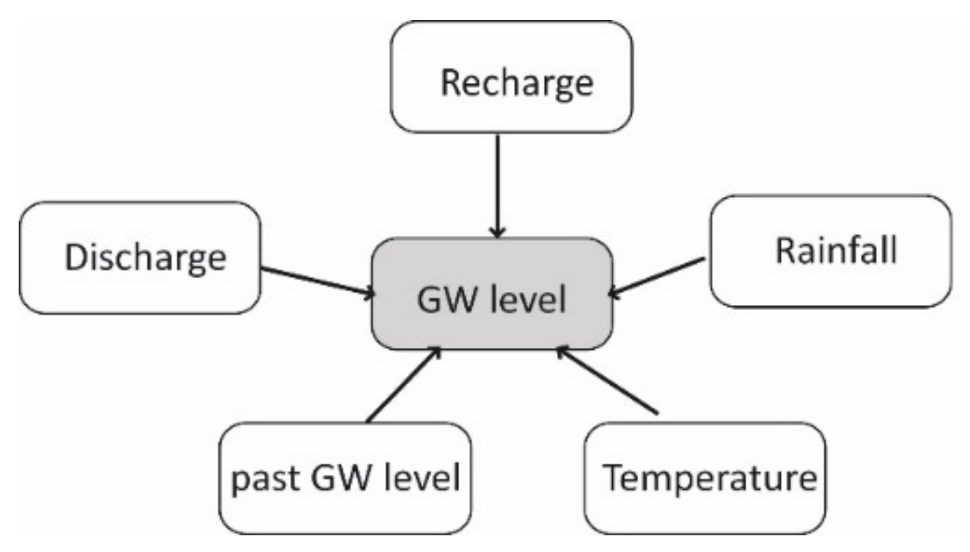
Figure 1. Example of the structure of a Bayesian model applied to groundwater-level study.

Connections define the conditional dependencies among variables (i.e., nodes) ^[29]. The dependencies are quantified by conditional probabilities for each node through a conditional table of probabilities. Usually, BNs are built by software that generates many network structures with the input parameters.

2.7. Instance-Based Weighting (IBW)

Instance-based algorithms derive from the nearest-neighbour pattern classifier ^[30], which is modified and extended by introducing a weighting function. IBW models are also inspired by exemplar-based models of categorisation ^[31]. Different from other machine learning algorithms, which return an explicit target function after learning from the training dataset, instance-based algorithms simply save the training dataset in memory ^[32]. For any new data, the algorithm first finds its n nearest neighbour in the training set and delays the processing effort until a new instance needs to be classified. IBW has many advantages such as the low training cost, the efficiency gained through solution reuse ^[33], ability to model complex target functions, and the capability to describe probabilistic concepts ^[34]. However, when irrelevant features are present, their performance decreases; an accurate distinction of relevant features can be achieved through feature weighting to ensure acceptable performance. IBW does not need to be trained and the results are less influenced by the training data size. Inverse-distance weighting is a special case of instance-based weighting with the weighting factor p = 2 ^[35].

2.8. Support Vector Machine (SVM)

SVM are kernel-based neural networks developed by Vapnik ^[36] to overcome the several weaknesses which affect the ANNs’ overall generalisation capability ^[37], including possibilities of getting trapped in local minima during training, overfitting the training data, and subjectivity in the choice of model architecture ^[38]. The SVM is based on statistical learning theory ^[39]; in particular, it is based on structural risk minimisation (SRM) instead of empirical risk minimisation (ERM) of ANNs. The SVM minimises the empirical error and model complexity simultaneously, which can improve the generalisation ability of the SVM for classification or regression problems in many disciplines. This is achieved by minimising an upper bound of the testing error rather than minimising the training error ^[32]; the solution of SVM with a well-defined kernel is always globally optimal, while many other machine learning tools (e.g., ANNs) are subjected to local optima; finally, the solution is represented sparsely by Supporting Vectors, which are typically a small subset of all training examples ^[40]. For further details, see refs. ^[15]^[39]^[41]^[42].

2.9. Decision Trees (DT)

Decision tree models ^[43] are based on the recursive division of the response data into many parts along any of the predictor variables in order to minimise the residual sum of squares (RSS) of the data within the resulting subgroups (i.e., “nodes” in the terminology of tree models) ^[44]. The number of nodes increases during the process of splitting along predictors. The tree-growing process stops when the within-node RSS is below a specified threshold or when a minimum specified number of observations within a node is reached ^[45]. However, the modeller places minimal limitations upon tree-fitting process, and fitted trees may be more complex than is actually warranted by the data available. The problem of overfitting results is then managed by the ‘pruning’ algorithms, which aid the modeller in the selection of a parsimonious description of interactions between response and predictors, fitting trees for the optimum structure for any level of complexity ^[44]. Because no prior assumptions are made about the nature of the relationships among predictors, and between predictors and response, decision trees are extremely flexible.

2.10. Random Forest (RF)

Random forests work by constructing groups of decision trees during the training process, representing a distinct instance of the classification of data input. Each tree is developed by independently sampling the values of a random vector with the same distribution for all trees in the forest ^[46].

The random forest technique considers the instances individually so that the trees are run in parallel; there is no interaction between these trees while building the trees. The prediction with the majority of votes or an average of the prediction is taken as the selected prediction (Figure 2). The RF algorithm was created to overcome the limitations of DT, reducing the overfitting of datasets and increasing prediction accuracy. The decision tree grows to the largest possible size without being pruned in accordance with the number of trees and the number of predictor variables ^[47].

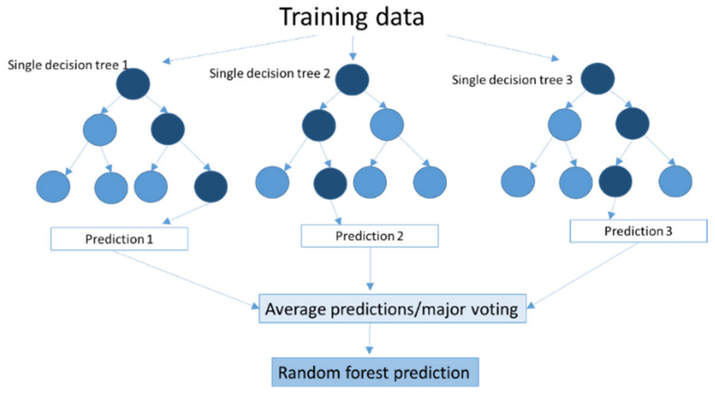
Figure 2. Scheme of Random Forest.

2.11. Gradient-Boosted Regression Trees (GBRT)

Gradient-Boosted Regression trees are ensemble techniques in which weak predictors are grouped together to enhance their performance ^[48]. Learning algorithms are combined in series to achieve a strong learner (“boosting”) from different weak learners (i.e., the decision trees) connected sequentially. Each tree attempts to minimise the errors of the previous tree. After the initial tree is generated from the data, subsequent trees are generated using the residuals from the previous tree. At each step, trees are weighted, with the lower-performing trees weighted the highest; this allows the improvement of performance at each iteration. A variety of loss functions can be used to detect the residuals.

References

Coppola, E., Jr.; Szidarovszky, F.; Poulton, M.; Charles, E. Artificial neural network approach for predicting transient water levels in a multilayered groundwater system under variable state, pumping, and climate conditions. J. Hydrol. Eng. 2003, 8, 348–360.
McDonald, M.G.; Harbaugh, A.W. A modular three-dimensional finite-difference ground-water flow model. In US Geological Survey Report 06-A1; US Geological Survey: Reston, VA, USA, 1988; p. 586.
Harbaugh, A.W.; Banta, E.R.; Hill, M.C.; Mcdonald, M.G. MODFLOW-2000, the US geological survey modular ground-water model—User guide to modularization concepts and the ground-water flow process. In US Geological Survey Open-File Report 00-92; US Geological Survey: Reston, VA, USA, 2000; p. 121.
Winston, R.B. MODFLOW-related freeware and shareware resources on the internet. Comput. Geosci. 1999, 25, 377–382.
Voss, C.I. A Finite-Element Simulation Model for Saturated–Unsaturated, Fluid-Density-dependent Ground-Water Flow with Energy Transport or Chemically Reactive Single-species. In Water-Resources Investigations Report 84-4369; US Geological Survey: Reston, VA, USA, 1984.
Babu, D.K.; Pinder, G.F. A finite element–finite difference alternating direction algorithm for 3- dimensional groundwater transport. Adv. Water Resour. 1984, 7, 116–119.
Bentley, L.R.; Kieper, G.M. Verification of the Princeton Transport Code (PTC). In Engineering Hydrology, Proceedings of the Symposium Sponsored by the Hydraulics Division of the American Society of Civil Engineers, San Francisco, CA, USA, 25–30 July 1993; American Society of Civil Engineers: New York, NY, USA, 1993; pp. 1037–1042.
Ewen, J.; Parkin, G.; O’Connell, P.E. SHETRAN: A coupled surface/subsurface modelling system for 3D water flow and sediment and solute transport in river basins. ASCE J. Hydrol. Eng. 2000, 5, 250–258.
Hsu, K.L.; Gupta, H.V.; Sorooshian, S. Artificial neural network modeling of the rainfall-runoff process. Water Resour. Res. 1995, 31, 2517–2530.
Schalkoff, R.J. Artificial Neural Networks; McGraw-Hill Higher Education: New York, NY, USA, 1997; p. 448.
Mohammadi, K. Groundwater Table Estimation Using MODFLOW and Artificial Neural Networks. In Practical Hydroinformatics; Abrahart, R.J., See, L.M., Solomatine, D.P., Eds.; Water Science and Technology Library: Springer: Berlin/Heidelberg, Germany, 2009; Volume 68.
Samarasinghe, S. Neural Networks for Applied Sciences and Engineering: From Fundamentals to Complex Pattern Recognition; Auerbach Publications: New York, NY, USA, 2016; ISBN 0429115784.
Taormina, R.; Chau, K.-W.; Sethi, R. Artificial neural network simulation of hourly groundwater levels in a coastal aquifer system of the Venice lagoon. Eng. Appl. Artifi. Intellig. 2012, 25, 1670–1676.
Wunsch, A.; Liesch, T.; Broda, S. Forecasting groundwater levels using nonlinear autoregressive networks with exogenous input (NARX). J. Hydrol. 2018, 567, 743–758.
Chen, C.; He, W.; Zhou, H.; Xue, Y.; Zhu, M. A comparative study among machine learning and numerical models for simulating groundwater dynamics in the Heihe River Basin, northwestern China. Sci. Rep. 2020, 10, 1–13.
Schwenker, F.; Kestler, H.A.; Palm, G. Three learning phases for radial-basis-function networks. Neural Netw. 2001, 14, 439–458.
Buhmann, M.D. Radial Basis Functions: Theory and Implementations; Cambridge University Press: Cambridge, UK, 2003; p. 258.
Kingston, G.B.; Maier, H.R.; Lambert, M.F. Calibration and validation of neural networks to ensure physically plausible hydrological modeling. J. Hydrol. 2005, 314, 158–176.
Jang, J.S.R. ANFIS adaptive-network-based fuzzy inference systems. IEEE Trans. Syst. Man. Cybern. 1993, 23, 665–685.
Kurtulus, B.; Razack, M. Modeling daily discharge responses of a large karstic aquifer using soft computing methods: Artificial neural network and neuro-fuzzy. J. Hydrol. 2010, 381, 101–111.
Almuhaylan, M.R.; Ghumman, A.R.; Al-Salamah, I.S.; Ahmad, A.; Ghazaw, Y.M.; Haider, H.; Shafiquzzaman, M. Evaluating the Impacts of Pumping on Aquifer Depletion in Arid Regions Using MODFLOW, ANFIS and ANN. Water 2020, 12, 2297.
Chen, S.H.; Lin, Y.H.; Chang, L.C.; Chang, F.J. The strategy of building a flood forecast model by neuro fuzzy network. Hydr. Proc. 2006, 20, 1525–1540.
Haykin, S. Communication Systems, 2nd ed.; Wiley: New York, NY, USA, 1994; pp. 45–90.
Saharia, M.; Bhattacharjya, R.K. Geomorphology-based time-lagged recurrent neural networks for runoff forecasting. KSCE J. Civ. Eng. 2012, 16, 862–869.
Sattari, M.; Taghi, K.Y.; Pal, M. Performance evaluation of artificial neural network approaches in forecasting reservoir inflow. Appl. Math. Model. 2012, 36, 2649–2657.
Huang, G.B.; Chen, L.; Siew, C.K. Universal approximation using incremental constructive feedforward networks with random hidden nodes. IEEE Trans. Neural Netw. 2006, 17, 879–892.
Huang, G.B.; Chen, L. Convex incremental extreme learning machine. Neurocomputing 2007, 70, 3056–3062.
Huang, G.B.; Chen, L. Enhanced random search based incremental extreme learning machine. Neurocomputing 2008, 71, 3460–3468.
Moghaddam, H.K.; Moghaddam, H.K.; Rahimzadeh Kivi, Z.; Bahreinimotlagh, M.; Javad Alizadeh, M. Developing comparative mathematic models, BN and ANN for forecasting of groundwater levels. Groundw. Sustain. Dev. 2019, 9, 100237.
Cleary, J.G.; Trigg, L.E. K*: An instance-based learner using an entropic distance measure. In Machine Learning, Proceedings of the Twelfth International Conference, San Francisco, CA, USA, 9–12 July 1995; Morgan Kaufmann Publishers Inc.: San Francisco, CA, USA, 1995; pp. 108–114.
Smith, E.E.; Medin, D.L. Categories and Concepts; Harvard University Press: Cambridge, MA, USA, 1981; p. 203.
Xu, T.; Valocchi, A.J.; Choi, J.; Amir, E. Use of machine learning methods to reduce predictive error of groundwater models. Groundwater 2014, 52, 448–460.
Aha, D.W. Feature Weighting for Lazy Learning algorithms. In Feature Extraction, Construction and Selection: A Data Mining Perspective; The American Statistical Association: Boston, MA, USA, 1998; Volume 1, p. 410.
Aha, D.W.; Kibler, D.; Albert, M.C. Instance-Based Learning Algorithms. Mach. Learn. 1991, 6, 37–66.
Michael, W.J.; Minsker, B.S.; Tcheng, D.; Valocchi, A.J.; Quinn, J.J. Integrating data sources to improve hydraulic head predictions: A hierarchical machine learning approach. Water Resour. Res. 2005, 41, 1–14.
Vapnik, V.N. The Nature of Statistical Learning Theory; Springer: New York, NY, USA, 1995; p. 314.
Gunn, S.R. Support vector machines for classification and regression. In ISIS Technical Report; University of Southampton: Southampton, UK, 1998; p. 66.
Demissie, Y.K.; Valocchi, A.J.; Minsker, B.S.; Bailey, B.A. Integrating a calibrated groundwater flow model with error-correcting data-driven models to improve predictions. J. Hydrol. 2009, 364, 257–271.
Yoon, H.; Jun, S.-C.; Hyun, Y.; Bae, G.-O.; Lee, K.-K. A comparative study of artificial neural networks and support vector machines for predicting groundwater levels in a coastal aquifer. J. Hydrol. 2011, 396, 128–138.
Cao, L.J.; Chua, K.S.; Chong, W.K.; Lee, H.P.; Gu, Q.M. A comparison of PCA, KPCA and ICA for dimensionality reduction in support vector machine. Neurocomputing 2003, 55, 321–336.
Vapnik, V.N. Statistical Learning Theory; John Wiley & Sons: New York, NY, USA, 1998; p. 768.
Smola, A.J.; Sch¨olkopf, B. A tutorial on support vector regression. Stat. Comput. 2004, 14, 199–222.
Quinlan, J.R. Induction of decision trees. Mach. Learn. 1986, 1, 81–106.
Breiman, L.; Friedman, J.H.; Olshen, R.A.; Stone, C.J. Classification and Regression Trees; Routhledge: New York, NY, USA, 1984; p. 368.
Anderton, S.P.; White, S.M.; Alvera, B. Evaluation of spatial variability of snow water equivalent in a high mountain catchment. Hydrol. Processes 2004, 18, 435–453.
Breiman, L. Random forests. Mach. Learn. 2001, 45, 5–32.
Aertsen, W.; Kint, V.; Van Orshoven, J.; Muys, B. Evaluation of Modelling Techniques for Forest Site Productivity Prediction in Contrasting Ecoregions Using Stochastic Multicriteria Acceptability Analysis (SMAA). Environ. Model. Softw. 2011, 26, 929–937.
Fienen, M.N.; Nolan, B.T.; Feinstein, D.T. Evaluating the sources of water to wells: Three techniques for metamodeling of a groundwater flow model. Environ. Model. Softw. 2016, 77, 95–107.

© Text is available under the terms and conditions of the Creative Commons Attribution (CC BY) license; additional terms may apply. By using this site, you agree to the Terms and Conditions and Privacy Policy.

Upload a video for this entry

Information

Subjects: Environmental Sciences

Contributor MDPI registered users' name will be linked to their SciProfiles pages. To register with us, please refer to https://encyclopedia.pub/register :

Cristina Di Salvo

View Times: 399

Update Date: 15 Aug 2022

Table of Contents

Video Upload Options

Confirm