Your browser does not fully support modern features. Please upgrade for a smoother experience.
Submitted Successfully!
 +1 credit
Thank you for your contribution! You can also upload a video entry or images related to this topic.
For video creation, please contact our Academic Video Service.
| Version | Summary | Created by | Modification | Content Size | Created at | Operation |
|---|---|---|---|---|---|---|
| 1 | Reza Khandan | + 1518 word(s) | 1518 | 2022-02-17 05:12:55 | | | |
| 2 | Jason Zhu | -3 word(s) | 1515 | 2022-02-18 03:10:42 | | | | |
| 3 | Jason Zhu | Meta information modification | 1515 | 2022-02-22 03:12:04 | | | | |
| 4 | Jason Zhu | -41 word(s) | 1474 | 2022-02-22 03:13:34 | | |
Video Upload Options
We provide professional Academic Video Service to translate complex research into visually appealing presentations. Would you like to try it?
Cite
If you have any further questions, please contact Encyclopedia Editorial Office.
Khandan, R. Assimilation of Key Data in Land Surface Models. Encyclopedia. Available online: https://encyclopedia.pub/entry/19606 (accessed on 21 June 2026).
Khandan R. Assimilation of Key Data in Land Surface Models. Encyclopedia. Available at: https://encyclopedia.pub/entry/19606. Accessed June 21, 2026.
Khandan, Reza. "Assimilation of Key Data in Land Surface Models" Encyclopedia, https://encyclopedia.pub/entry/19606 (accessed June 21, 2026).
Khandan, R. (2022, February 17). Assimilation of Key Data in Land Surface Models. In Encyclopedia. https://encyclopedia.pub/entry/19606
Khandan, Reza. "Assimilation of Key Data in Land Surface Models." Encyclopedia. Web. 17 February, 2022.
Copy Citation
The correction of Soil Moisture (SM) estimates in Land Surface Models (LSMs) is considered essential for improving the performance of numerical weather forecasting and hydrologic models used in weather and climate studies. Along with surface screen-level variables, the satellite data, including Brightness Temperature (BT) from passive microwave sensors, and retrieved SM from active, passive, or combined active–passive sensor products have been used as two critical inputs in improvements of the LSM.
Soil Moisture (SM)
Land Surface Models
Brightness Temperature
1. Introduction
Soil Moisture (SM) is a crucial variable in the partitioning of water (into infiltration and runoff) and energy (into sensible and latent heat flux) and has been considered in many atmospheric and hydrological studies [1][2]. SM influences the carbon cycling by photosynthesis and transpiration processes [3] and affects short and medium-range forecasts in meteorology [4]. The variability in SM is due to the spatial distribution of many factors such as rainfall, the spatial variation of the soil texture, vegetation, and topography. Volumetric SM measurements at different depths are limited to sparse ground measurements, which cannot provide required spatial and temporal resolution data for numerical weather initialization. To solve this problem, Land Surface Models (LSMs) are used to model the near-surface (~0–5 cm) and root zone (~5 to 100) SM (hereafter referred to as SSM and RSM) behavior through physical and hydrological laws. However, the estimation of SM by LSMs is limited by forcing data, built-in physical rules, and parameterizations.
In order to reduce the mentioned uncertainties, the assimilation of surface observations in LSMs was proposed. Generally, the assimilation procedure in LSMs consists of three main components: (i) observation, (ii) modeling (LSM) for background and forecast generation of SM, and (iii) correction of background SM in the LSM based on observations. As stated in [5], the initial assimilation experiments based on the optimal interpolation method used screen-level temperature and relative humidity as assimilation inputs. However, this approach had some built-in limitations, such as applied fix coefficients, the accumulation of errors induced by the model, forcing data in the root zone, and sparse data sampling [5][6][7].
The emergence of satellite data both in the infrared and microwave spectrum has made it possible to measure the Brightness Temperature (BT) and to estimate volumetric SMs at the near surface (SSM). Such observations can be applied as an external source for the correction of biases in SM initialization in LSMs. For this purpose, microwave imaging sensors (both passive and active) have been more desirable due to their low attenuation by clouds and atmospheric aerosols [8]. The passive sensors include: Soil Moisture Active and Passive (SMAP) radiometer (L-band 1.41 GHz) [9]; Soil Moisture and Ocean Salinity (SMOS) (L-band 1.4 GHz) [10]; Advanced Microwave Scanning Radiometer–Earth Observing System (AMSR-E) (C, X, K, Ka, and W bands at six frequencies: 6.93, 10.65, 18.7, 23.8, 36.5, and 89.0 GHz) [11]; Advanced Microwave Scanning Radiometer 2 (AMSR2) (C, X, K, Ka, and W bands at seven frequencies: 6.93, 7.3, 10.65, 18.7, 23.8, 36.5, and 89 GHz) [12][13][14]; Scanning Multichannel Microwave Radiometer (SMMR) (C, X, K, and Ka bands at five frequencies: 6.6, 10.7, 18.0, 21.0, and 37.0 GHz) [15]; and Tropical Rainfall Measuring Mission’s (TRMM) Microwave Imager (TMI) (X, K, Ka, and W bands at five frequencies 10.7, 19.4, 21.3, 37.0, and 85.5 GHz) [16]. The active sensors include: Advanced Scatterometer (ASCAT) (C-band 5.255 GHz) [13]; Sentinel-1 (C-band 5.405 GHz) [14]; and ERS Scatterometer (C-band 5.32 GHz) [17]. The merged products of these sensors, Climate Change Initiative (CCI) [18] and Soil Moisture Operational Products System (SMOPS) [19], can also be applied for such assimilation studies.
A successful assimilation procedure depends on the assimilation approach, LSM physical laws and parameterizations, the Radiative Transfer Model (RTM) parameterization (as an observation operator for BT), and the observations and errors in both the model and observations [20][21]. The theoretical issues about the assimilation of both satellite BT and SM were discussed in [20][22][23]. As miscellaneous papers used different satellite data, LSMs, data preparation, forcing data, assimilation approaches (with different settings), observation operators (RTM), and different locations, it is helpful to normalize and summarize their results for future studies.
2. The Results of Assimilating BT and SM in LSMs
Figure 1 and Figure 2 compare the performance of non-assimilation cases with respect to assimilation cases based on bias (Figure 1A), correlation (Figure 1B), RMSE (Figure 1C), and unbiased RMSE (uRMSE) (Figure 1D) computed between the SM estimated in LSM and ground SM networks for SSM and RSM, respectively. Non-assimilation cases include those bias-corrected/non-bias corrected. In Figure 1A, which shows the bias for NOAH, Jules, and VIC, the SM bias range varies between −0.096 and 0.13 (m3 m-3) for non-assimilation studies and between −0.077 and 0.069 (m3 m-3) for assimilation studies. The NOAH has the greater variability in both cases, with assimilation cases having lower biases. In Figure 1B, the performances of NOAH, CLSM, CLM, Jules, ISBA, SiB2, and VIC are shown for a correlation index. The correlation varies between −0.243 and 0.95 in non-assimilations and between 0.343 and 0.93 for assimilations. The mean of assimilation (0.69) cases is higher than non-assimilation (0.64) cases.
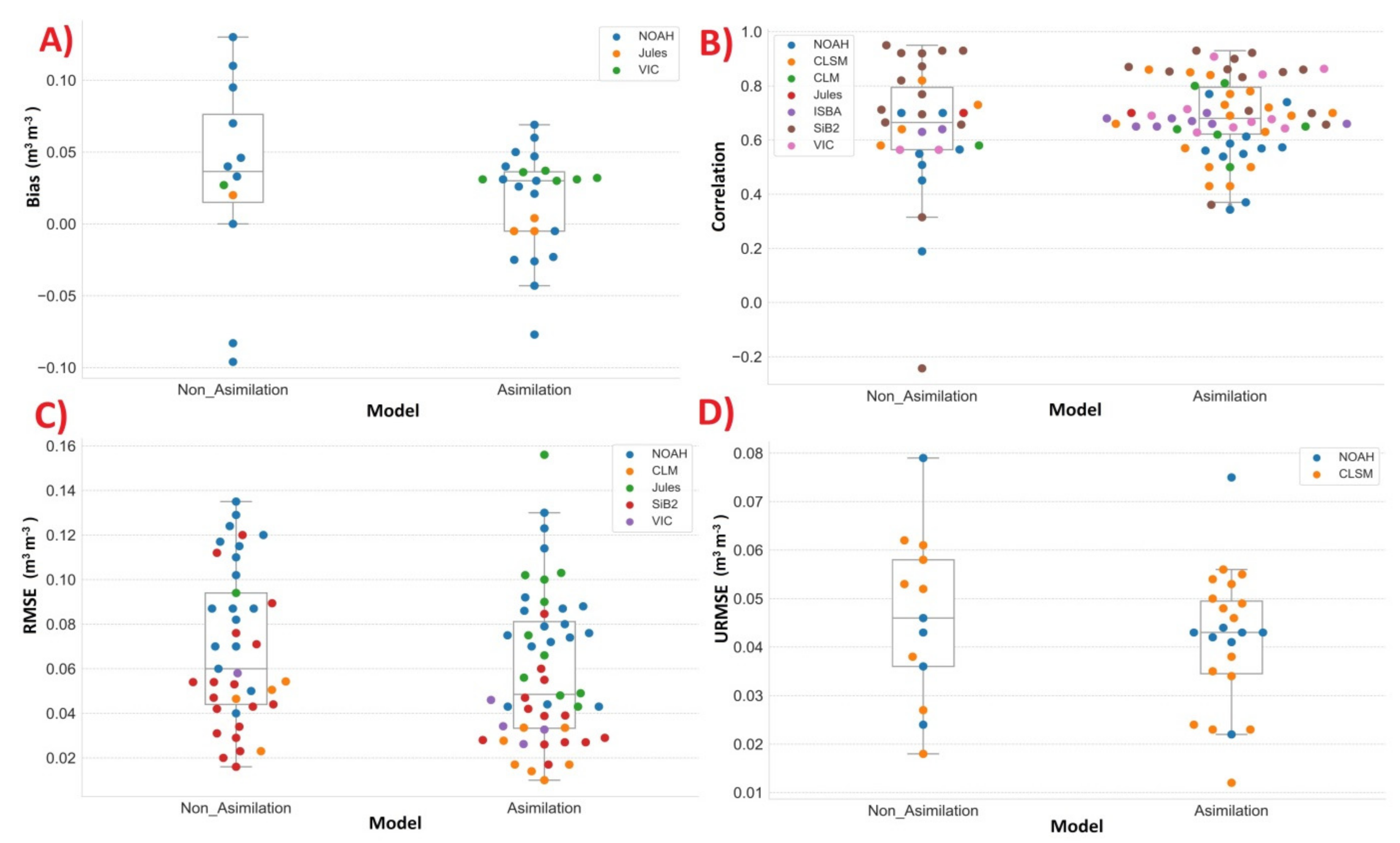
Figure 1. Assimilation results for SSM: (A) bias (m3 m-3), (B) correlation, (C) RMSE (m3 m-3), and (D) uRMSE (m3 m-3); the metrics are computed based on estimated SM in LSMs and ground networks.
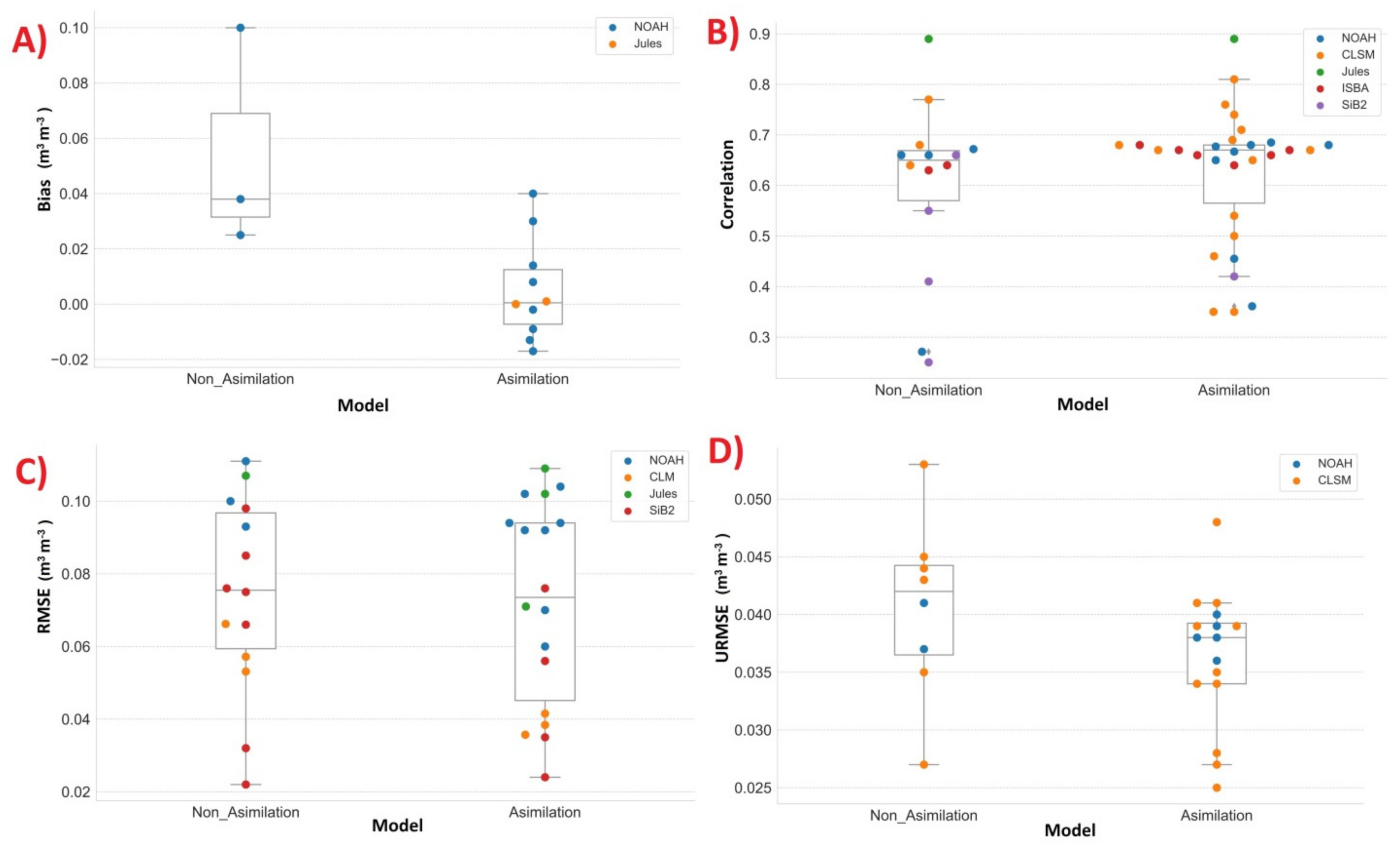
Figure 2. Assimilation results for RSM: (A) bias (m3 m-3), (B) correlation, (C) RMSE (m3 m-3), and (D) uRMSE (m3 m-3); the metrics are computed based on estimated SM in LSMs and ground networks.
In Figure 1C, the RMSE in NOAH, CLM, Jules, SiB2, and VIC varies between 0.016 and 0.13 (m3 m-3) in non-assimilation cases and between 0.01 and 0.15 (m3 m-3) for assimilation cases. The mean of RMSE (0.058 m3 m-3) is lower in assimilation cases with respect to non-assimilations (0.069 m3 m-3). In Figure 1D, the uRMSE in NOAH and CLSM varies between 0.018 and 0.079 (m3 m-3) in non-assimilations and between 0.012 and 0.075 (m3 m-3) in assimilations. The uRMSE mean of assimilations (0.041 m3 m-3) is lower than non-assimilations (0.046 m3 m-3).
Figure 2 is the same as Figure 1 but regarding RSM. In Figure 2A, the performances of NOAH and Jules in the bias index are shown. The range for non-assimilation cases varies between 0.025 and 0.1 (m3 m-3) and between −0.017 and 0.04 (m3 m-3) for assimilation cases. The mean for assimilation cases (0.005 m3 m-3) is lower compared with non-assimilation cases (0.054 m3 m-3). In Figure 2B, the correlations for NOAH, CLSM, Jules, ISBA, and SiB2 are shown. The ranges vary between 0.25 and 0.89 in non-assimilations and between 0.35 and 0.89 in assimilations. In Figure 2C, the RMSE is shown for NOAH, CLM, Jules, and SiB2, varying between 0.022 and 0.111 (m3 m-3) for non-assimilations and between 0.024 and 0.109 (m3 m-3) for assimilations. In Figure 2D, the uRMSE is shown for NOAH and CLSM. The ranges vary between 0.027 and 0.053 (m3 m-3) for non-assimilations and between 0.025 and 0.048 (m3 m-3) for assimilations. The uRMSE mean of assimilations (0.036 m3 m-3) is lower than that of non-assimilations (0.040 m3 m-3). Such results (both in SSM and RSM) are shown to demonstrate the quantitative range of error indices in the reviewed papers. These ranges are a function of many factors, such as the accuracy of in situ measurements, study area, the applied sensors, assimilation methods, etc.
To show the effect of the assimilation procedures, the differences between assimilation and non-assimilation cases are reported (sorted based on correlation) for SSM (Figure 3). Some researchers conducted multiple approaches, which are shown as slots with different colors in each bar; for example, [24] conducted two assimilation scenarios with different configurations. As Figure 3 shows, most of assimilation approaches improved the SM estimation. In some papers [24][25][26], some configurations resulted in negative correlation differences where only one station was used, which cannot be considered a robust result.
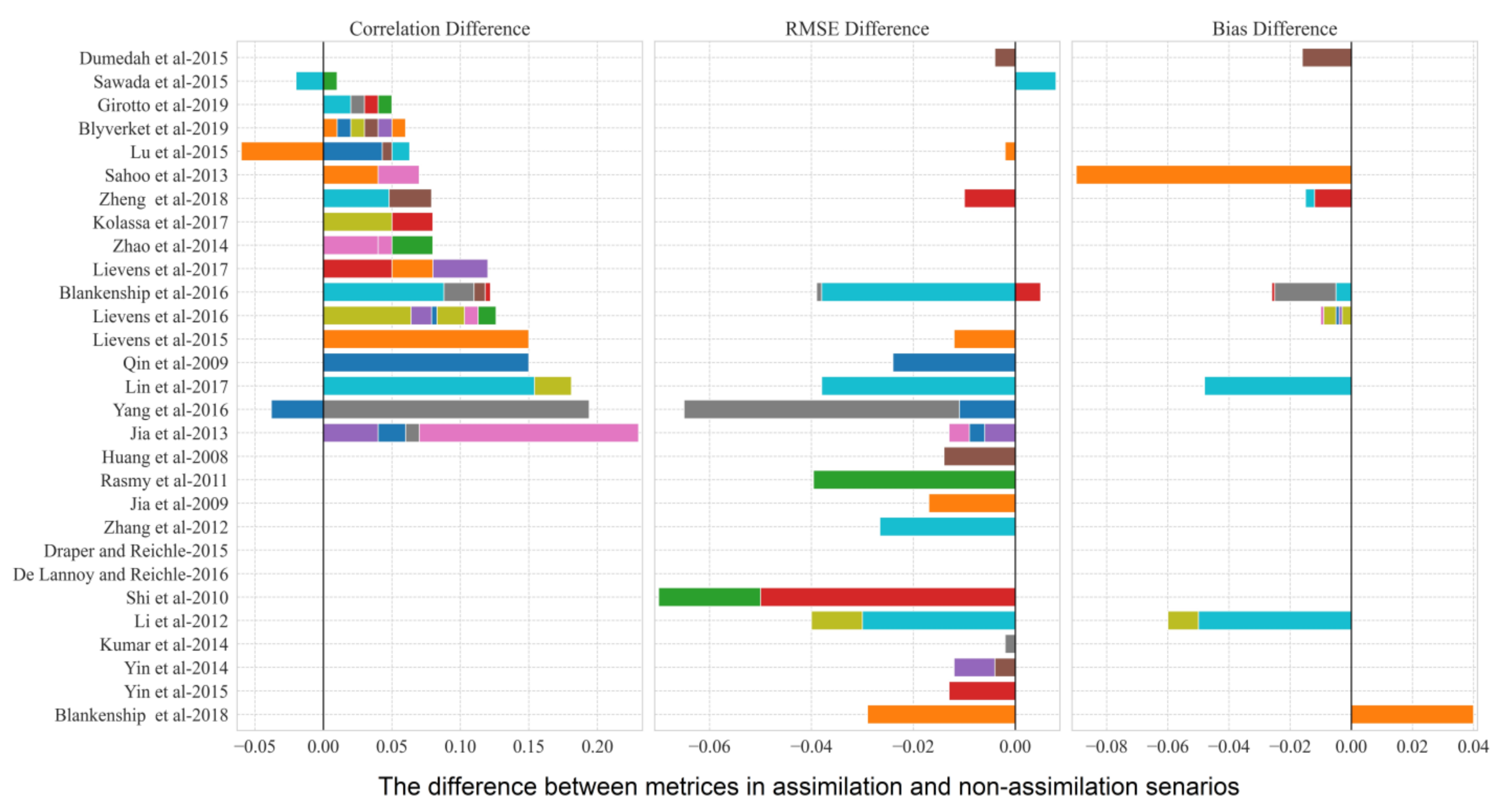
Figure 3. The difference between metrics in assimilation and non-assimilation scenarios for SSM in terms of correlation, bias, and RMSE; the y axis shows the authors of papers, and the three columns show the metrics.
Most of these scenarios used AMSR-E and SMOS in their assimilation studies. Overall, when BT and SM are used as input, no significant priority can be found between them. The highest improvement was observed in [27] with CLM LSM and the En4DVAR approach in China. Most configurations used EnKF for conducting the assimilation.
Based on Figure 3, RMSE improvements for assimilation cases vary between −0.002 and −0.07 (m3 m-3) (excluding positive values of retrogression).
In Figure 4, the improvements in correlation, RMSE, and bias are shown for RSM. In most cases, the correlation was improved. The correlation improvements vary between 0.005 and 0.184 (excluding negative values). In [24], a significant negative correlation was found, which is the subtraction of assimilation from open loop (the open loop is initialized with 35 days of assimilation results). It shows that when the Sib2 LSM was initialized with 35 days of assimilation, better results were obtained, and the open-loop run in this configuration had better performance than assimilation in the whole study period. Regarding RMSE, most of the studies reported an improvement between −0.007 and −0.04 (m3 m-3) (excluding positive values). All available studies show bias improvements in RSM by assimilation.
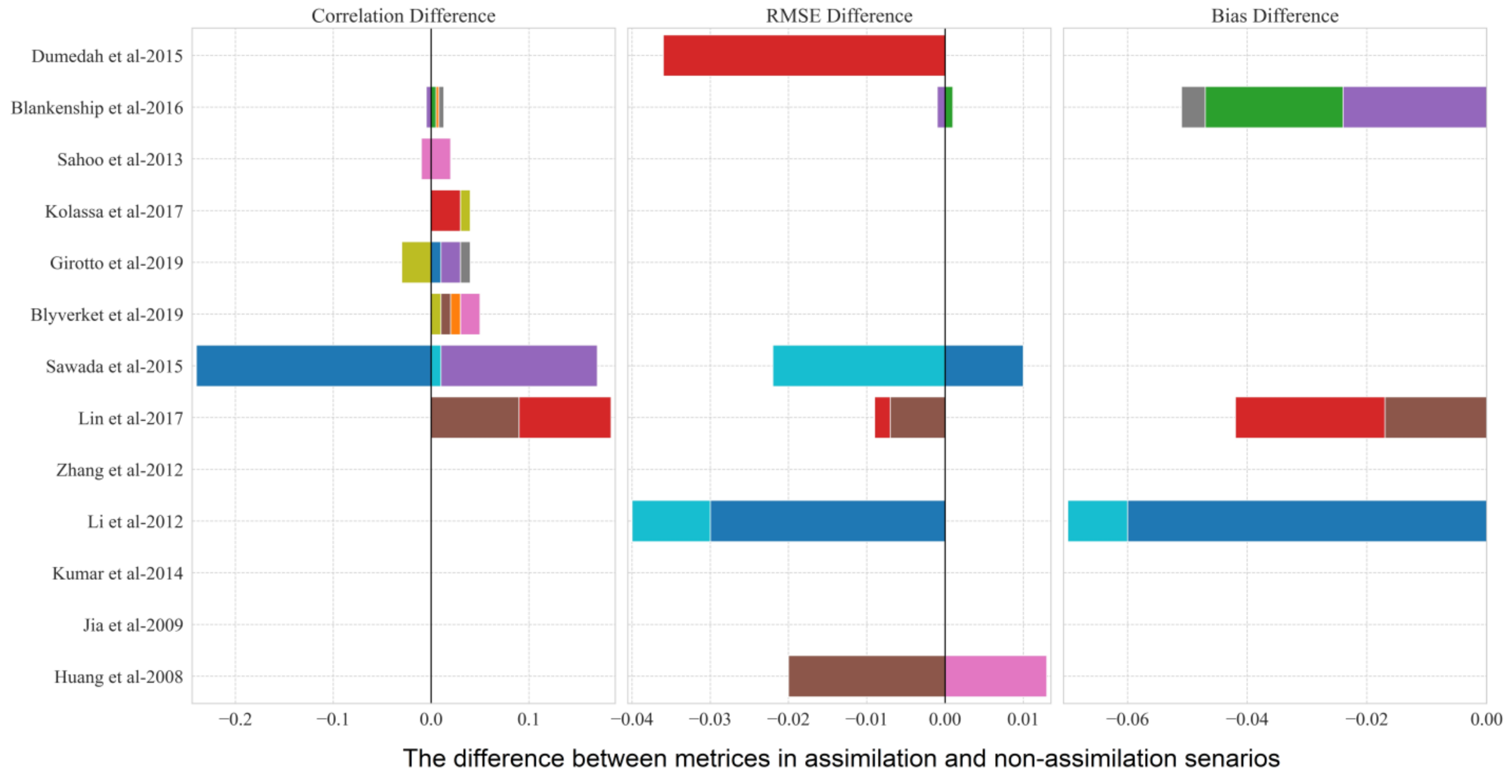
Figure 4. The difference between metrics in assimilation and non-assimilation scenarios for RSM: bias (m3 m-3), correlation, RMSE (m3 m-3), and uRMSE (m3 m-3); the y axis shows the authors of papers, and the three columns show the metrics.
References
- Loew, A. Impact of surface heterogeneity on surface soil moisture retrievals from passive microwave data at the regional scale: The Upper Danube case. Remote Sens. Environ. 2008, 112, 231–248.
- Seneviratne, S.I.; Corti, T.; Davin, E.L.; Hirschi, M.; Jaeger, E.B.; Lehner, I.; Orlowsky, B.; Teuling, A.J. Investigating soil moisture–climate interactions in a changing climate: A review. Earth-Sci. Rev. 2010, 99, 125–161.
- van der Molen, M.K.; Dolman, A.J.; Ciais, P.; Eglin, T.; Gobron, N.; Law, B.E.; Meir, P.; Peters, W.; Phillips, O.L.; Reichstein, M.; et al. Drought and ecosystem carbon cycling. Agric. For. Meteorol. 2011, 151, 765–773.
- Rasmy, M.; Koike, T.; Boussetta, S.; Lu, H.; Li, X. Development of a satellite land data assimilation system coupled with a mesoscale model in the Tibetan Plateau. IEEE Trans. Geosci. Remote Sens. 2011, 49, 2847–2862.
- De Rosnay, P.; Drusch, M.; Vasiljevic, D.; Balsamo, G.; Albergel, C.; Isaksen, L. A simplified Extended Kalman Filter for the global operational soil moisture analysis at ECMWF. Q. J. R. Meteorol. Soc. 2013, 139, 1199–1213.
- Mahfouf, J.F.; Bergaoui, K.; Draper, C.; Bouyssel, F.; Taillefer, F.; Taseva, L. A comparison of two off-line soil analysis schemes for assimilation of screen level observations. J. Geophys. Res. Atmos. 2009, 114, D08105.
- de Rosnay, P.; Balsamo, G.; Albergel, C.; Muñoz-Sabater, J.; Isaksen, L. Initialisation of land surface variables for numerical weather prediction. Surv. Geophys. 2014, 35, 607–621.
- Petropoulos, G.P.; Ireland, G.; Barrett, B. Surface soil moisture retrievals from remote sensing: Current status, products & future trends. Phys. Chem. Earth Parts A/B/C 2015, 83, 36–56.
- Entekhabi, D.; Njoku, E.G.; O’Neill, P.E.; Kellogg, K.H.; Crow, W.T.; Edelstein, W.N.; Entin, J.K.; Goodman, S.D.; Jackson, T.J.; Johnson, J.; et al. The soil moisture active passive (SMAP) mission. Proc. IEEE 2010, 98, 704–716.
- Kerr, Y.H.; Waldteufel, P.; Richaume, P.; Wigneron, J.P.; Ferrazzoli, P.; Mahmoodi, A.; Al Bitar, A.; Cabot, F.; Gruhier, C.; Juglea, S.E.; et al. The SMOS soil moisture retrieval algorithm. IEEE Trans. Geosci. Remote Sens. 2012, 50, 1384–1403.
- Njoku, E.G.; Jackson, T.J.; Lakshmi, V.; Chan, T.K.; Nghiem, S.V. Soil moisture retrieval from AMSR-E. IEEE Trans. Geosci. Remote Sens. 2003, 41, 215–229.
- Imaoka, K.; Kachi, M.; Kasahara, M.; Ito, N.; Nakagawa, K.; Oki, T. Instrument performance and calibration of AMSR-E and AMSR2. Int. Arch. Photogramm. Remote Sens. Spat. Inf. Sci. 2010, 38, 13–18.
- Wagner, W.; Hahn, S.; Kidd, R.; Melzer, T.; Bartalis, Z.; Hasenauer, S.; Figa-Saldana, J.; De Rosnay, P.; Jann, A.; Schneider, S.; et al. The ASCAT soil moisture product: A review of its specifications, validation results, and emerging applications. Meteorol. Z. 2013, 22, 5–33.
- Paloscia, S.; Pettinato, S.; Santi, E.; Notarnicola, C.; Pasolli, L.; Reppucci, A. Soil moisture mapping using Sentinel-1 images: Algorithm and preliminary validation. Remote Sens. Environ. 2013, 134, 234–248.
- Njoku, E.G.; Stacey, J.; Barath, F.T. The Seasat scanning multichannel microwave radiometer (SMMR): Instrument description and performance. IEEE J. Ocean. Eng. 1980, 5, 100–115.
- Gao, H.; Wood, E.F.; Jackson, T.; Drusch, M.; Bindlish, R. Using TRMM/TMI to retrieve surface soil moisture over the southern United States from 1998 to 2002. J. Hydrometeorol. 2006, 7, 23–38.
- Wagner, W.; Lemoine, G.; Rott, H. A method for estimating soil moisture from ERS scatterometer and soil data. Remote Sens. Environ. 1999, 70, 191–207.
- Dorigo, W.; Wagner, W.; Albergel, C.; Albrecht, F.; Balsamo, G.; Brocca, L.; Chung, D.; Ertl, M.; Forkel, M.; Gruber, A.; et al. ESA CCI Soil Moisture for improved Earth system understanding: State-of-the art and future directions. Remote Sens. Environ. 2017, 203, 185–215.
- Liu, J.; Zhan, X.; Hain, C.; Yin, J.; Fang, L.; Li, Z.; Zhao, L. NOAA soil moisture operational product system (SMOPS) and its validations. In Proceedings of the 2016 IEEE International Geoscience and Remote Sensing Symposium (IGARSS), Beijing, China, 10–15 July 2016; pp. 3477–3480.
- De Lannoy, G.J.M.; de Rosnay, P.; Reichle, R.H. Soil moisture data assimilation. In Handbook of Hydrometeorological Ensemble Forecasting; Springer: Berlin/Heidelberg, Germany, 2016; pp. 1–43.
- De Lannoy, G.J.; Reichle, R.H.; Vrugt, J.A. Uncertainty quantification of GEOS-5 L-band radiative transfer model parameters using Bayesian inference and SMOS observations. Remote Sens. Environ. 2014, 148, 146–157.
- Maggioni, V.; Houser, P.R. Soil moisture data assimilation. In Data Assimilation for Atmospheric, Oceanic and Hydrologic Applications; Springer: Berlin/Heidelberg, Germany, 2017; Volume 3, pp. 195–217.
- Montzka, C. Soil Moisture Remote Sensing and Data Assimilation. In Remote Sensing of Energy Fluxes and Soil Moisture Content; CRC Press: Boca Raton, FL, USA, 2013; pp. 415–434.
- Sawada, Y.; Koike, T.; Walker, J.P. A land data assimilation system for simultaneous simulation of soil moisture and vegetation dynamics. J. Geophys. Res. Atmos. 2015, 120, 5910–5930.
- Lu, H.; Yang, K.; Koike, T.; Zhao, L.; Qin, J. An improvement of the radiative transfer model component of a land data assimilation system and its validation on different land characteristics. Remote Sens. 2015, 7, 6358–6379.
- Yang, K.; Zhu, L.; Chen, Y.; Zhao, L.; Qin, J.; Lu, H.; Tang, W.; Han, M.; Ding, B.; Fang, N. Land surface model calibration through microwave data assimilation for improving soil moisture simulations. J. Hydrol. 2016, 533, 266–276.
- Jia, B.; Tian, X.; Xie, Z.; Liu, J.; Shi, C. Assimilation of microwave brightness temperature in a land data assimilation system with multi-observation operators. J. Geophys. Res. Atmos. 2013, 118, 3972–3985.
More
Information
Subjects:
Remote Sensing; Meteorology & Atmospheric Sciences
Contributor
MDPI registered users' name will be linked to their SciProfiles pages. To register with us, please refer to https://encyclopedia.pub/register
:
View Times:
1.0K
Entry Collection:
Environmental Sciences
Revisions:
4 times
(View History)
Update Date:
22 Feb 2022
Table of Contents


Notice
You are not a member of the advisory board for this topic. If you want to update advisory board member profile, please contact office@encyclopedia.pub.
OK
Confirm
Only members of the Encyclopedia advisory board for this topic are allowed to note entries. Would you like to become an advisory board member of the Encyclopedia?
Yes
No
${ textCharacter }/${ maxCharacter }
Submit
Cancel
Back
Comments
${ item }
|
${ item.createdUser.fullName }
${ item.createdAt }
${ item.vote }
${ item.reply }
Delete
${ reply.createdUser.fullName }
${ reply.createdAt }
${ reply.vote }
Delete
There is no reply to this comment~
${ item.replyTextCharacter }/${ item.replyMaxCharacter }
Submit
Cancel
More
No more~
There is no comment~
${ textCharacter }/${ maxCharacter }
Submit
Cancel
${ selectedItem.replyTextCharacter }/${ selectedItem.replyMaxCharacter }
Submit
Cancel
Confirm
Are you sure to Delete?
Yes
No