Optical Diffraction Tomography

Version	Summary	Created by	Modification	Content Size	Created at	Operation
1		Ahmed Bassam Ayoub	+ 1444 word(s)	1444	2022-01-21 08:01:17	\|
2	format correct	Conner Chen	+ 33 word(s)	1477	2022-01-28 02:47:08	\|

This entry is adapted from the peer-reviewed paper 10.3390/app12030951

Optical Diffraction Tomography (ODT) is an emerging tool for label-free imaging of semi-transparent samples in three-dimensional space. Being semi-transparent, such objects do not strongly alter the amplitude of the illuminating field.

optical diffraction tomography ODT

1. Introduction

Optical Diffraction Tomography (ODT) is an emerging tool for label-free imaging of semi-transparent samples in three-dimensional space ^[1]^[2]^[3]^[4]^[5]^[6]^[7]^[8]^[9]^[10]. Being semi-transparent, such objects do not strongly alter the amplitude of the illuminating field. However, the total phase delay at a particular wavelength is a function of the refractive index of the sample and also the thickness of the sample. Due to this ambiguity, one cannot distinguish between those parameters from 2D projections. Hence, to reconstruct the 3D refractive index (RI) map of semi-transparent samples, a holographic detection is needed to extract the phase of the field after passing through the sample. Then, by acquiring different holograms at different illumination angles, the 3D RI map can be reconstructed using inverse scattering models ^[10].

Holographic detection was introduced by Gabor who used “in-line” holography. He showed that the intensity image retrieved from the in-line holography is composed of an “in-focus” image in addition to an “out-of-focus” image (i.e., “Twin” image) ^[11]. Due to this “Twin” image problem, in-line holography usually encounters problems in retrieving the phase of the object. Upatnieks and Leith proposed an “off-axis” holography ^[12]. In this configuration, a small tilt is introduced between the reference arm and the sample arm, which results in shifting in the Fourier domain the “out-of-focus” image with respect to the “in-focus”. Since then, “off-axis” interferometry has been widely used in ODT by first extracting the phase before using the inverse models ^[13]^[14].

2. Theory

The intensity pattern captured by the detector of the ODT system is denoted by It(x,y) with x and y being the horizontal and the vertical dimensions of the 2D intensity pattern. The detected intensity is given by:

I_{t} = {|U_{i}|}^{2} + {|U_{s}|}^{2} + 2 |U_{i}| |U_{s}| \cos (φ_{s} - φ_{i})

(1)

where |Ui| is the amplitude of the incident field, |Us| is the amplitude of the scattered field, and φs−φi is the difference between the phases of the complex scattered and the incident field, carrying the phase information of the sample. For weakly scattering samples (i.e., Born approximation), we can assume that (|Us|<<|Ui|), and defining Ui=ejφi,∣∣Ui∣∣=1, Equation (1) can be simplified as follows:

I_{t} \approx 1 + 2 |U_{s}| \cos (Δ φ)

(2)

where Δφ = φs−φi. Equation (2) can be rewritten as:

\begin{array}{l} I_{t} = 1 + 2 |U_{s}| \cos (Δ ϕ) \\ \Rightarrow I_{t} = 1 + |U_{s}| e^{j Δ ϕ} + |U_{s}| e^{- j Δ ϕ} \end{array}

(3)

Multiplying both sides of Equation (3) by Ei=ejϕi, we obtain:

\begin{array}{l} I_{t} e^{j φ_{i}} & = |U_{s}| e^{j φ_{s}} + e^{j φ_{i}} + |U_{s}| e^{- j φ_{s}} e^{2 j φ_{i}} \\ = U_{s} + e^{j φ_{i}} + U_{s}^{*} e^{2 j φ_{i}} \\ = U_{s} + e^{j φ_{i}} (1 + U_{s}^{*} e^{j φ_{i}}) \end{array}

(4)

Equation (4) includes the effect of the scattered field (i.e.,Us), which we refer to as the “Principal” image and its complex conjugate (i.e.,Us∗), which we refer to as the twin image. As has been shown previously ^[15], at illumination angles less than the numerical aperture, the two terms tend to cancel each other, which results in a low contrast 3D reconstruction while maintaining the high frequency features of the sample. Figure 1 shows the effect of changing the illumination angle on the 2D intensity image of a simulated digital phantom where different illumination angles were assumed. Note the 2D Fourier transform of the corresponding intensity images includes two circles in the Fourier domain. Each circle is the result of the spectral filtering applied by the limited numerical aperture of the objective lens. From Equation (3), we see that we have three terms: a Zero-order term (the first term on the right-hand side) and the two cross terms. The shift of the two circles from the Zero-order term depends on the illumination angle of the incident plane wave.

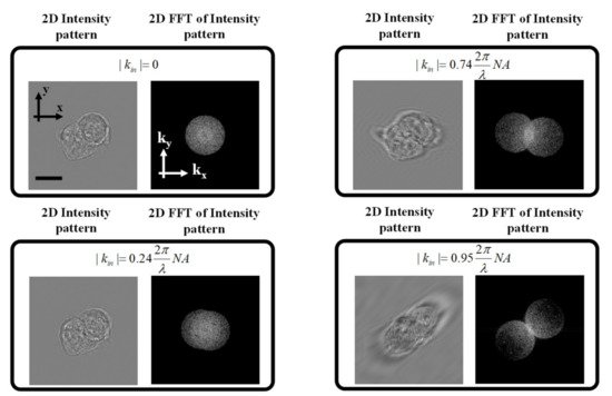
Figure 1. Intensity images and their 2D Fourier transforms for on-axis and off-axis configurations with different illumination angles. As can be seen from the figures, as the incident illumination vector kin approaches the numerical aperture of the objective lens, the 2 cross terms can be decoupled, and the principal term can be retrieved. Scale bar = 8 μm.

In other words, for normal incidence, the two circles completely overlap with each other. However, as we increase the illumination angle, the shift between the two circles increases until we reach the limit of the numerical aperture, at which point we see that the two circles are tangent to each other. Only when the illumination is at the maximum angle permitted by the NA of the objective lens can the complex field be retrieved from the intensity image as would be the case for an off-axis interferometric setup with a separate reference arm for holographic detection.

Figure 1 shows that for an accurate extraction of the scattered field, the sample should be illuminated with the maximum angle permitted by the NA of the objective lens ^[16]. The scattered field can be extracted by simply multiplying the intensity measurement with the incident plane wave, which results in shifting the spectrum in the Fourier domain. This is followed by the spatial filtering of the “Principal” image with a circular filter whose size is determined by the NA of the objective lens as shown in Figure 2.

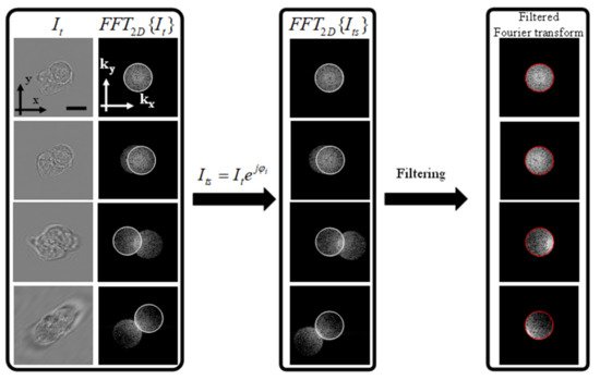
Figure 2. Processing of the 2D intensity images before mapping into the 3D Fourier space. The left-most panel shows the intensity measurements and the corresponding Fourier transform. The middle panel shows the effect of multiplying by the incident plane wave, which results in centering the scattered field highlighted by the white circles. The final step is the filtering of the scattered field with a circular filter whose size matches the size of the numerical aperture in the Fourier space declared by the red circle. Scale bar = 8 μm.

From Figure 2, it can be seen that only when the illumination angle is at the edge of the imaging NA can we extract the complex scattered field from the intensity image. This can be experimentally demonstrated by illumination along a circular cone whose center is perfectly aligned with the imaging objective lens. This is demonstrated in the experimental setup described in the following section.

By multiplying the intensity image with the incident plane-wave to shift the spectrum in the Fourier domain, the scattered field spectrum becomes centered around the origin. To filter out the complex scattered field in the Fourier domain, we apply a low pass filter given by the following equation:

{\tilde{U}}_{s} (k_{x}, k_{y}) = L P F {F F T_{2 D} {I_{t} e^{j φ_{i}}}}

(5)

where U˜s(kx,ky) is the 2D Fourier transform of Us(x,y), and LPF{.} represents a circular low pass filter whose radius is given by k0NA, where k0 is the wave number in free-space.

By extracting the complex field along the direction k=(kx,ky,kz) for each illumination k-vector kin=(kinx,kiny,kinz), one Fourier component of the 3D spectrum of the scattering potential F˜(κ→) (which is directly related to the index distribution) can be retrieved ^[1]:

\tilde{F} (\vec{κ}) = \frac{k_{z}}{2 π j} {\tilde{U}}_{s} (k_{x}, k_{y})

(6)

where

\vec{κ} = \vec{k} - {\vec{k}}_{i} = {[\begin{array}{l} k_{x} - k_{x}^{i n} \\ k_{y} - k_{z}^{i n} \\ \sqrt{{(k_{0} n_{0})}^{2} - k_{x}^{2} - k_{y}^{2}} - k_{z}^{i n} \end{array}]}_{}

where κ→ is the 3D spatial frequency of the scattering potential, k0=2πλ, λ is the wavelength of the illumination beam, and n0 is the refractive index of the surrounding medium. We refer to Equation (6) as the Wolf transform ^[1]^[17].

By applying Equation (6) for different 2D projections and accumulating the various spectral components in the 3D Fourier domain, the 3D spectrum F˜(κ→) can be measured. Subsequently, F(r) can be spatially reconstructed using an inverse 3D Fourier transform. Finally, n(r) is retrieved using the following equation:

n (r) = \sqrt{\frac{4 π}{k_{0}^{2}} F (r) + n_{0}^{2}}

(7)

In summary, we obtain the 3D RI distribution, through the following steps; (1) the raw images should be processed to remove the background; (2) the illumination angle is calculated; (3) the intensity image is multiplied with the incident plane-wave to shift the scattered field spectrum to the center; (4) the resulting spectrum is low pass filtered with a circular filter whose radius is proportional to the numerical aperture of the imaging objective lens; (5) the resulting low pass filtered spectrum is mapped to the 3D Fourier space of the sample as a spherical cap (i.e., diffraction); (6) by applying steps 1–5 for all intensity images with different illumination angles, the 3D scattering potential is formed in the 3D Fourier space; and (7) by applying an inverse 3D Fourier transform, the spatial distribution of the scattering potential is calculated from which the 3D RI distribution is retrieved.

Preprocessing of the images is performed by subtracting the background from the raw images to remove any noise from the camera or the ambient environment. The background is retrieved by applying a low pass filter onto the raw images. The normalized intensity profile is then calculated as follows:

I_{n} = \frac{I_{t} - I_{B k g}}{I_{B k g}}

(8)

where IBkg is the background signal.

References

Wolf, E. Three-dimensional structure determination of semi-transparent objects from holographic data. Opt. Commun. 1969, 1, 153–156.
Sung, Y.; Choi, W.; Fang-Yen, C.; Badizadegan, K.; Dasari, R.R.; Feld, M.S. Optical diffraction tomography for high resolution live cell imaging. Opt. Express 2009, 17, 266–277.
Haeberlé, O.; Belkebir, K.; Giovaninni, H.; Sentenac, A. Tomographic diffractive microscopy: Basics, techniques and perspectives. J. Mod. Opt. 2010, 57, 686–699.
Sung, Y.; Choi, W.; Lue, N.; Dasari, R.R.; Yaqoob, Z. Stain-Free Quantification of Chromosomes in Live Cells Using Regularized Tomographic Phase Microscopy. PLoS ONE 2012, 7, e49502.
Kim, T.; Zhou, R.; Goddard, L.L.; Popescu, G. Solving inverse scattering problems in biological samples by quantitative phase imaging. Laser Photon. Rev. 2016, 10, 13–39.
Shin, S.; Kim, K.; Yoon, J.; Park, Y. Active illumination using a digital micromirror device for quantitative phase imaging. Opt. Lett. 2015, 40, 5407–5410.
Charrière, F.; Marian, A.; Montfort, F.; Kühn, J.; Colomb, T.; Cuche, E.; Marquet, P.; Depeursinge, C. Cell refractive index tomography by digital holographic microscopy. Opt. Lett. 2006, 31, 178–180.
Cooper, K.L.; Oh, S.; Sung, Y.; Dasari, R.R.; Kirschner, M.W.; Tabin, C.J. Multiple phases of chondrocyte enlargement underlie differences in skeletal proportions. Nature 2013, 495, 375–378.
Choi, W.; Fang-Yen, C.; Badizadegan, K.; Oh, S.; Lue, N.; Dasari, R.R.; Feld, M.S. Tomographic phase microscopy. Nat. Methods 2007, 4, 717–719.
Slaney, M.; Kak, A.; Larsen, L. Limitations of Imaging with First-Order Diffraction Tomography. IEEE Trans. Microw. Theory Tech. 1984, 32, 860–874.
Gabor, D. A New Microscopic Principle. Nature 1948, 161, 777–778.
Leith, E.N.; Upatnieks, J. Reconstructed Wavefronts and Communication Theory. J. Opt. Soc. Am. 1962, 52, 1123–1128.
Boas, D.A.; Pitris, C.; Ramanujam, N. (Eds.) Handbook of Biomedical Optics; CRC Press: Boca Raton, FL, USA, 2016.
Cuche, E.; Bevilacqua, F.; Depeursinge, C. Digital holography for quantitative phase-contrast imaging. Opt. Lett. 1999, 24, 291–293.
Ayoub, A.B.; Lim, J.; Antoine, E.E.; Psaltis, D. 3D reconstruction of weakly scattering objects from 2D intensity-only measurements using the Wolf transform. Opt. Express 2021, 29, 3976–3984.
Li, J.; Matlock, A.; Li, Y.; Chen, Q.; Zuo, C.; Tian, L. High-speed in vitro intensity diffraction tomography. Adv. Photon. 2019, 1, 066004.
Born, M.; Wolf, E. Principles of Optics: Electromagnetic Theory of Propagation, Interference and Diffraction of Light, 7th ed.; Cambridge University Press: Cambridge, UK, 1999.

© Text is available under the terms and conditions of the Creative Commons Attribution (CC BY) license; additional terms may apply. By using this site, you agree to the Terms and Conditions and Privacy Policy.

Upload a video for this entry

Information

Subjects: Acoustics

Contributor MDPI registered users' name will be linked to their SciProfiles pages. To register with us, please refer to https://encyclopedia.pub/register :

Ahmed Bassam Ayoub

View Times: 1.8K

Update Date: 28 Jan 2022

Table of Contents

Video Upload Options

Confirm

1. Introduction

2. Theory

References