Deep Learning in Deconvolution Problem

Version	Summary	Created by	Modification	Content Size	Created at	Operation
1		Mikhail A. Makarkin	+ 3992 word(s)	3992	2021-12-21 09:21:09	\|
2	Done	Jason Zhu	Meta information modification	3992	2021-12-24 10:02:21	\|

This entry is adapted from the peer-reviewed paper 10.3390/mi12121558

In modern digital microscopy, deconvolution methods are widely used to eliminate a number of image defects and increase resolution.

Deconvolution Deep Learning Machine learning

1. Deconvolution Types

The works mentioned above use the well-known point spread function (PSF) of the optical system. The PSF describes the imaging system’s response to the infinitely small object (single point size). The PSF of an imaging system can be measured using the small calibration objects of the known shape or calculated from the first principles if researchers know the parameters of the imaging system. Therefore, these and similar methods are classified as non-blind deconvolution methods. However, more often than not, the PSF cannot be accurately calculated for several reasons. First, it is impossible to take into account all the noise and distortions that arise during shooting. Second, the PSF can be very complex in shape. Alternatively, the PSF can change during the experiment ^[1]^[2]. Therefore, methods have been developed that extract the estimated PSF directly from the resulting images. These methods can be either iterative (the PSF estimate is obtained from a set of parameters of sequentially obtained images that are refined at each pass of the algorithm) or non-iterative (the PSF is calculated immediately by some parameters and metrics of one image).

The mathematical formulation of the blind deconvolution problem is a very ill-posed problem and can have a large (or infinite) number of solutions ^[3]. Therefore, it is still necessary to impose certain restrictions on the condition—to introduce regularization, for example, in the form of a so-called penalty block, such as a kernel intensity penalizer ^[4] or a structured common least norm ^[5] (STLN), or in other ways. A typical problem, in this case, is the appearance of image artifacts ^[6]^[7], which appear due to an insufficiently accurate PSF estimate or because of the nature of the noise. This problem is especially acute for iterative deconvolution methods, since there is a possibility that PSF and noise in different images will not coincide with real ones, and therefore the error accumulates at each iteration (Figure 1). In this regard, machine learning algorithms are of particular interest because they are specifically geared towards extracting information from data and their iterative processing.

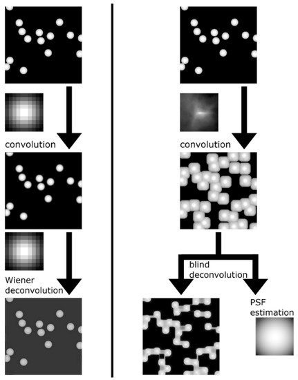
Figure 1. Difference between blind and non-blind deconvolution. On the left is an example of convolution and non-blind deconvolution with the same kernel and some regularization. On the right is an example of poor estimation of PSF with blind deconvolution. A generated image of the same-shaped objects similar to an atomic force microscopy (AFM) image is used as the source. A real AFM tip shape is used as a convolution kernel in this case. Blind deconvolution based on the Villarrubia algorithm ^[8] confuses object shape and tip shape, resulting in poor image restoration.

An important issue when solving the deconvolution problem is the nature of the distortion. It can be uniform (that is, the same distortion kernel and/or noise is applied to all parts of the image) or non-uniform (different blur kernels are applied to different parts of the image and/or the noise on them is also not the same). The absence of a uniform distortion for the image further complicates the task. In these cases, it is no longer possible to proceed with a general estimate that researchers derive from large-scale dependencies between pixels. Instead, researchers have to consider local dependencies in small areas of the image, which makes global dependencies more complex structures in a mathematical sense, and much more expensive from a purely computational perspective. Figure 2 shows an example of a non-uniform blur. Accordingly, different types of distortion must be applied to different deconvolution types, either uniform or non-uniform. In the future, researchers will use as synonyms the concepts of homogeneous and uniform, heterogeneous and non-uniform.

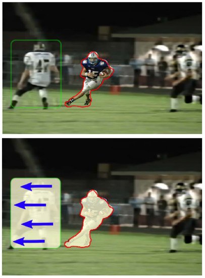
Figure 2. An example of non-uniform distortion. Image is taken from ^[9]. The operator tracks and focuses on the player with the ball, so there is no blur for his image and the small area around him (red outline). The area indicated by the green outline will show slight defocusing distortion and motion blur (direction of movement is shown by arrows). To adequately restore such an image, it will be necessary to establish the relationships between such areas and consider the transitions between them.

In real-life problems, one must confront the problem of inhomogeneous distortions most often.

2. Application of Deep Learning in a Deconvolution Problem

Machine learning is divided into classical (ML) and deep learning (DL). Classical algorithms are based on manual feature selection or construction. Deep learning transfers the task of feature construction entirely to the neural network. This approach allows the process to be fully automated and performs blind deconvolution in the complete sense, i.e., restoring images only using information from the initial dataset. Therefore, the solution to the deconvolution problem using DL is an auspicious direction at the moment. The automation of feature extraction allows these algorithms to be adapted to the variety of resulting images, which is crucial since it is almost impossible to obtain an accurate PSF estimate and reconstruct an image by using it in the presence of random noise and/or several types of parameterized noise. A more reasonable solution would be to build its iterative approximation, which will adjust when the input data changes, as DL does. Today, two main neural network types are used for deconvolution.

The first is convolutional neural networks (CNN). In CNN, alternating convolutional and downsampling layers extract from the image a set of spatially invariant hierarchical features, a set of low-level geometric shapes, and transformations of pixels that line up into specific high-level features ^[10]. In theory, in the presence of “blurred/non-blurred image” pairs, CNN can learn a specific set of transformations for image pixels that lead to blur (i.e., evaluate the PSF) (Figure 3 and Figure 4). For example, in ^[11], the authors show that, on the one hand, such considerations are relevant; on the other hand, they do not work well for standard CNN architectures and do not always produce a sharp image. The reason is that small kernels are used for convolutions. Because of this, the network is unable to find correlations between far-apart pixels.

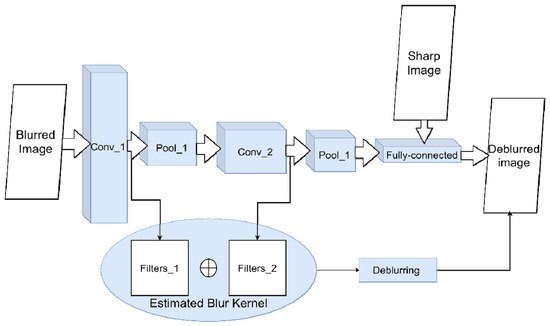
Figure 3. Scheme for image deconvolution with kernel blur using CNN. To solve the classification problem of a blurred/non-blurred image, the neural network adjusts its weights and filters in convolutional layers during training. The sequence of applied filters will be approximately equivalent to the blur kernel.

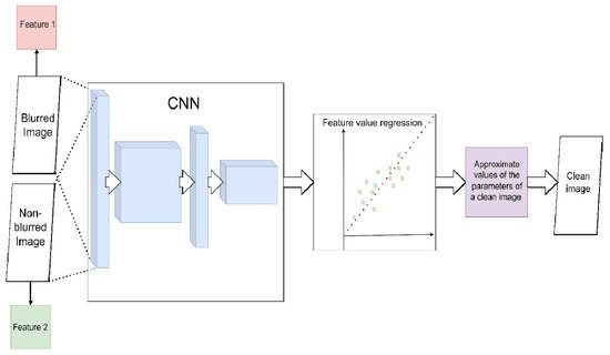
Figure 4. Scheme for image deconvolution with image-to-image regression using CNN (without PSF estimation). CNN directly solves the regression problem with the spatial parameters of the images. The parameters of the blurred image (red) are approximated to the parameters of the non-blurred (green). The resulting estimate is used to restore a clean image.

Nevertheless, using CNNs for image restoration problems leads to the appearance of artifacts. The simple replacement of small kernels with large kernels in convolutions does not generally allow the network to be trained due to the explosion of gradients. Therefore, the authors replaced the standard convolutions with the pseudoinverse kernel of the discrete Fourier transform function. This kernel is chosen so that it can be decomposed into a small number of one-dimensional filters. Standard Wiener deconvolution is used for initial activation, which improves the restored image’s sharpness.

However, the convolution problem is not the only one. When using the classic CNN architectures (AlexNet ^[12], VGG ^[13]), researchers have found that they perform poorly at reconstructing images with non-uniform backgrounds, often leaving certain areas of the image blurry. One can often find such a phenomenon as the fluctuation of blur during training—under the same conditions and on the same data, with frozen weights, the network after training still gives both sharp and blurry images. What seems paradoxical is that an increase in the training sample number and an increase in the depth of the model led to the fact that the network began to recover images with blur more often. This is due to some properties of the CNN architectures, primarily the use of standard loss functions. As shown in ^[14]^[15], blur primarily suppresses high-frequency areas in the image (which means that the L-norms of the images decrease). This means that with the standard maximum a posteriori approach (MAP) with an error function that minimizes the L₁ or L₂ norm, the optimum of these functions will correspond to a blurry image, not a sharp one. As a result, the network learns to produce blurry images. Some modification of the regularization can partially suppress this effect, but this is not a reliable solution. In addition, the estimation for minimizing the distance between the true and blurred image is inconvenient because, if there are strongly and weakly blurred images in the sample, neural networks are trained to display intermediate values of blur parameters. Thus, they either underestimate or overestimate blur ^[16]. Therefore, using CNN for the deconvolution task requires specific additional steps.

The use of multiscale learning looks promising in this regard (Figure 5). To obtain a clean image after deconvolution, researchers need to solve two problems. First, find local patterns on small patches so that small details can be restored. Second, consider the interaction between far-apart pixels to capture the distortion pattern typical to the image. This requires the network to extract spatial features from multiple image scales. It also helps to learn how these traits will change as the resolution changes. In ref. ^[17], the authors propose using a neural network architecture called CRCNN (concatenated residual convolutional neural network). In this approach, residual blocks are used as the elements of spatial feature extraction in an implicit form and are then fed into an iterative deconvolution (IRD) algorithm. They are then concatenated at the output to obtain multiscale deconvolution. In addition, the approach described in ^[18] integrates the encoder-decoder architecture (see, for example, ^[19]) and recurrent blocks. A distorted image at different scales is fed into the input of the network. When training a network, the weights from the network’s branches for smaller scales are reused, with the help of the residual connection when training branches for larger ones. This reduces the number of parameters and makes learning easier. Another important advantage of multiscale learning is the ability to completely abandon the kernel assessment and end-to-end modeling of a clear image. The general idea ^[20] is that co-learning the network at different scales and establishing a connection between them using modified residual blocks allows a fully-fledged regression to be carried out. researchers are not looking for the blur kernel, but approximating a clear image in spatial terms (for example, the intensity of the pixels at a specific location in an image). At the moment, the direction of using multiscale training looks promising, and other exciting results have already been obtained in ^[21]^[22]^[23]. Researchers can separately note an attempt to use the attention mechanism to study the relationship between spatial objects and the channels on an image ^[24].

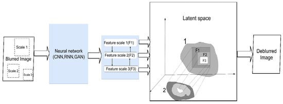
Figure 5. Principle of multiscale learning. A neural network of any suitable architecture extracts spatial features at different scales (F1, F2, F3) of the image. In various ways, smaller-scale features are used in conjunction with larger-scale features. This makes it possible to build an approximate explicit, spatially consistent clean image (2) from the latent representation of a clean picture (1).

The second type of architecture used is generative models, which primarily includes various modifications of generative adversarial networks (GANs) ^[25]. Generative models try to express a pure latent image explicitly. Information about it is implicitly contained in the function space (Figure 6). GAN training is closely related to the previous issue discussed above: prioritization and the related training adjustments. The work ^[26] used two pre-trained generative models to create non-blurred images and synthetic blur kernels. Next, grids were used to approximate the real kernel of the blur using a third, untrained generator. In ref. ^[27], a special class network—spatially constrained generative adversarial network (SCGAN) ^[28]—was used, which can directly isolate spatial features in the latent space and manipulate them directly. This feature made it possible to modify it for training on sets of images projected along three axes, implementing their joint deconvolution, and obtaining a sharp three-dimensional image. When using GAN, the problem of the appearance of image artifacts almost always plays a unique role. At the beginning of the training cycle, the network has to make strong assumptions about the nature of the noise (for instance, Gaussian, Poisson) and its uniform distribution across all of the images. The article ^[29] proposes eradicating artifacts without resorting to additional a priori constraints or additional processing. The authors set up a convolutional network as a generator and trained it to produce sharp images with its error function independently. At the same time, there remained a common error function for the entire GAN, which affected setting the minimax optimization. A simplified VGG was taken as a generator, which determined whether the input image was real or not. As a result, CNN and GAN worked together. The generator updated its internal variable directly to reduce the error between x and G(z). The GAN then updated the internal variable to produce a more realistic output.

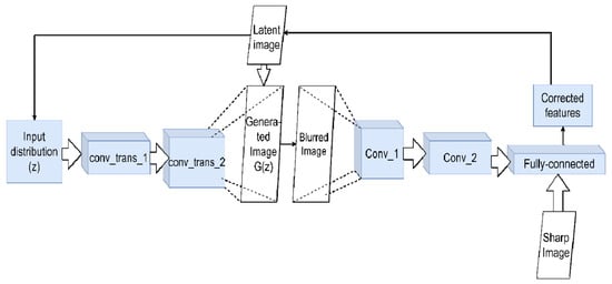
Figure 6. Using GAN for deconvolution. The generator network creates a false image G(z) from the initial distribution z (at first, it may be just noise). It is fed to the input of the network discriminator, which should distinguish it from the present. The discriminator network is trained to distinguish between blurred and non-blurred images, adjusting the feature values accordingly. These values form the control signal for the main generator. This signal will change G(z) step by step to approach the latent clean image iteratively.

The general problems affecting blind deconvolution are still present while using a DL approach, albeit with their own specificities. Blind deconvolution is an inverse problem that still requires sufficiently strong prior constraints, explicit or implicit, to work (Figure 7). As an example of explicit constraints, one can cite the above assumptions about the homogeneity of noise in images, the assumption that optical aberrations are described by Zernike polynomials ^[30], or directly through special regularizing terms ^[31]. A good example of implicit constraints is the pretraining generator networks in a GAN or the training discriminator networks that use certain blurry/sharp images sets. These actions automatically determine the specific distribution in the response space corresponding to the training data. According to this distribution, control signals are generated and supplied to the generator. It will adjust to this distribution and produce an appropriate set of synthetic PSFs or parameters for a clean image. This approach allows extracting prior constraints directly from the data. This property is typical for generative models in general; for example, the combination of an asymmetric autoencoder with end-to-end connections and a fully connected neural network (FCN) is used in ^[32]. The autoencoder creates a latent representation of the clean image, and the FCN learns to extract the blur kernels from the noise and serves as an additional regularizer for the autoencoder. The coordinated interaction of these networks makes it possible to reduce the deconvolution problem, contributing to a MAP optimization of the network parameters.

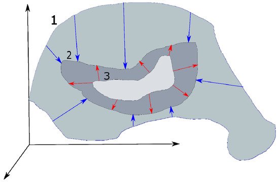
Figure 7. The principle of using the prior constraints. It narrows the infinite set of all possible values of the parameters of image 1 to the final one. Stronger prior constraints allow the narrowing of this set more precisely to the one corresponding to the true pure image 2 (shown by blue arrows). In turn, a more accurate and flexible model will iteratively refine its estimate of the clean image 3 (depicted by red arrows).

The clear advantages of the neural network approach include the already mentioned full automation, the ability to use the end-to-end pipeline (which significantly simplifies the operation and debugging of the method, or its modification if necessary), and its high accuracy. The disadvantages include problems common to DL—the need for sufficiently large and diverse datasets for training and computational complexity (especially for modern CNN and GAN architectures). However, it is worth highlighting the weak interpretability of the results—even with the deconvolution problem, it is often necessary to restore the image, estimate the PSF, and understand how it was obtained.

In addition to GAN and CNN, other architectures are used for the deconvolution problem. An autoencoder consists of two connected neural networks—an encoder and a decoder. The encoder takes input data and transforms it, making the representation more compact and concise. In the generating subtype, the variational autoencoder, the encoder part produces not one vector of hidden states but two vectors—mean values and standard deviations—according to which the data will be restored from random values. In addition to ^[32], the article ^[33] can be noted. It uses the output of a denoising autoencoder, which is typically the local average of the true density of the natural image, while the error of the autoencoder is the vector of the mean shift. With a known degradation, it is possible to iteratively decrease the value of the average shift and bring the solution closer to the average value, which is supposed to be cleaned of distortions. In the article ^[34], an autoencoder was used to find invariants on a clean/blurry image, based on which the GAN was trained to restore clean images. Autoencoders are commonly used to remove noise by transforming and compressing data ^[35]^[36]^[37].

For the case of video (when there is a sequential set of slightly differing images), some type of recurrent neural network (RNN) is often used, most often in combination with CNN. In work ^[38], individual CNN's first obtained the pixel weights of the incoming images from the dynamic scene and extracted its features. The four RNNs then processed each performance map (one for each direction of travel), and then the result was combined by the final convolutional network. This helped increase the receptive field and ensured that spatial non-uniformity of the blur was taken into account. In work ^[39], based on the convLSTM blocks, a pyramidal model of the interpolation of blurred images was built, which provided continuous interpolation of the intermediate frames, building an averaged sharp frame, and distributing information about it to all modules of the pyramid. This created an iterative de-blurring process. An interesting approach is proposed in ^[40], which offers an alternative to multiscale learning, called multi-temporal learning. It does not restore a clean image at small scales then go to the original resolution but rather works in a temporal resolution. A strong blur is a set of weak blurs that are successive over time. With the help of the RNN, the correction of weak initial blurring is iterated over the entire time scale.

Interest in the use of attention mechanisms in the task of deconvolution is beginning to grow. Attention in neural networks allows one to concentrate the processing of incoming information on its most important parts and establish a certain hierarchy of relations between objects to each other (initially, attention mechanisms were developed in the field of natural language processing and helped to determine the context of the words used). Attention mechanisms can be implemented as separate blocks in classical architectures and used, for example, to store and further summarize global information from different channels ^[41] or to combine hierarchical functions from different points in time in a video in a similar way ^[42]. Attempts are being made to use an architecture entirely based on attention—the so-called transformers ^[43]. An illustrative example of their use is shown in ^[44]. The authors take advantage of one of the main advantages of the transformer—the ability to handle global dependencies. Using residual links and building the architecture in a similar Y-net style allows the user to obtain local dependencies and link them to larger ones. As mentioned above regarding multiscale learning, this is one of the main problems in image deconvolution and, perhaps, the attention mechanism will allow one to solve it more efficiently—in some tasks (for example, removing rain and moiré patterns), the increase in PSNR and SSIM is very noticeable.

Deep learning is also beginning to be widely used in microscopy and related techniques. Yang et al. showed an example of non-blind deconvolution by using neural networks for 3D microscopy with different viewing angles for samples ^[45]. Usually, CNNs have some difficulty recognizing rotations, so the authors used GANs with a self-controlled approach to learning. It allowed them to surpass the standard algorithms for three-dimensional microscopy (CBIF ^[46], EBMD ^[47]) in terms of quantitative and qualitative characteristics: PSNR (peak signal-noise ratio), SSIM (structural similarity index), and CC (correlation coefficients). The flexibility of deep learning can also be seen in ^[48], which shows how it can be combined with the classical method. In this work, adaptive filters were used with the Wiener—Kolmogorov algorithm. The neural network predicted the optimal values of the regularizer and adjusted the filter kernel for it. It helped to improve the quality of the resulting image. In this case, the computational time was less than with direct image restoration using neural network training. It is an important point—in microscopy, especially in imaging cytometry, a transition to real-time image processing is needed. Examples can be given where super-resolution is achieved using the GAN ^[49]^[50], the encoder-decoder ^[51], and the U-Net-based architectures ^[52]. The use of deep learning in these works made it possible to significantly improve the quality of the reconstructed image and remove the connection to the optical properties of the installations, reducing the problem to a purely computational one. Despite the demanding computational power of deep learning algorithms, against the background of classical methods (especially nonlinear ones), they can show excellent performance ^[53] precisely due to their ability to build hierarchical features. Their other feature is the need for large datasets for training. On the one hand, the need is satiated by the appearance of large databases of cellular images in the public domain; on the other hand, it is still a problem. However, in imaging flow cytometry, a large dataset is relatively easy to collect. Therefore, it is convenient to use neural networks in flow cytometry with visualization; for example, the residual dense network can be used to eradicate blurring ^[54].

The use of deep learning made it possible to cope with non-uniform distortion, which classical methods could hardly achieve, and therefore weakened the requirements for the quality of the restored images. In addition to increasing the numerical characteristics, deep learning allows one to automate the image recovery process thoroughly and, therefore, expand its use for non-specialist users.

Furthermore, deep learning is used in medical imaging, by which researchers mean here all non-microscopic instruments (e.g., CT, MRI, and ultrasound). In ref. ^[55], a standard approach was used to extract the main features of images with a convolutional network at a low resolution and restore a pure image at a higher resolution. A similar but slightly complicated method is shown in ^[56], where the so-called upsampling layer was additionally used in the network architecture (the terminology requires caution: the layer was previously called the deconvolution layer, but it did not perform the deconvolution operation and this caused confusion). The methods were tested on MRI and retinal images. Chen et al. proposed adding residual bandwidth to the U-net encoder/decoder network to improve the quality of low-dose CT scans ^[57]. The encoder branch reduces noise and artifacts, and the decoder recovers structural information in the CT image. In addition, a residual gap-filling mechanism will complement the details lost when going through multiple layers of convolution and deconvolution. Finally, in ^[58], the convolutional network was trained to recognize the difference between low- and high-resolution MRI heart slices, and then taught to use this information as a recovery operator.

Deep learning is being used to improve image quality in photography and video. In addition to the usual adaptation of algorithms to, for example, mobile devices (see the review ^[59]), it can also be found being applied to the restoration of old photographs ^[60] or shooting fast-moving objects ^[61].

Moreover, deep learning deconvolution is used in astronomy ^[62]^[63]^[64]. In this area, observations are inevitably prone to distortion due to the presence of the atmosphere. In addition, they are often inhomogeneous due to the turbulence of the air masses, so the use of DL helps a lot.

References

Izeddin, I.; El Beheiry, M.; Andilla, J.; Ciepielewski, D.; Darzacq, X.; Dahan, M. PSF Shaping Using Adaptive Optics for Three-Dimensional Single-Molecule Super-Resolution Imaging and Tracking. Opt. Express 2012, 20, 4957.
Cremers, D.; Magnor, M.; Oswald, M.R.; Zelnik-Manor, L. (Eds.) Video Processing and Computational Video. In Lecture Notes in Computer Science; Springer: Berlin/Heidelberg, Germany, 2011; Volume 7082, ISBN 978-3-642-24869-6.
Kotera, J.; Smidl, V.; Sroubek, F. Blind Deconvolution with Model Discrepancies. IEEE Trans. Image Process. 2017, 26, 2533–2544.
Keuper, M.; Temerinac-Ott, M.; Padeken, J.; Heun, P.; Brox, T.; Burkhardt, H.; Ronneberger, O. Blind Deconvolution with PSF Regularization for Wide-Field Microscopy. In Proceedings of the 2012 9th IEEE International Symposium on Biomedical Imaging (ISBI), Barcelona, Spain, 2–5 May 2012; pp. 1292–1295.
Guo, H.; Renaut, R.A. A Regularized Total Least Squares Algorithm. In Total Least Squares and Errors-in-Variables Modeling; Springer: Dordrecht, The Netherlands, 2002; pp. 57–66.
Mosleh, A.; Langlois, J.M.P.; Green, P. Image Deconvolution Ringing Artifact Detection and Removal via PSF Frequency Analysis. In Lecture Notes in Computer Science, Proceedings of the Computer Vision—ECCV 2014, Zurich, Switzerland, 6–12 September 2014; Fleet, D., Pajdla, T., Schiele, B., Tuytelaars, T., Eds.; Springer: Cham, Switzerland, 2014; Volume 8692, pp. 247–262.
Meiniel, W.; Angelini, E.; Olivo-Marin, J.-C. Image Denoising by Adaptive Compressed Sensing Reconstructions and Fusions; Papadakis, M., Goyal, V.K., Van De Ville, D., Eds.; Proceedings of SPIE.: Bellingham, WA, USA, 2015; p. 95970X.
Villarrubia, J.S. Algorithms for Scanned Probe Microscope Image Simulation, Surface Reconstruction, and Tip Estimation. J. Res. Natl. Inst. Stand. Technol. 1997, 102, 425.
Bahat, Y.; Efrat, N.; Irani, M. Non-Uniform Blind Deblurring by Reblurring. In Proceedings of the IEEE International Conference on Computer Vision (ICCV), Venice, Italy, 22–29 October 2017; pp. 3286–3294.
Lecun, Y.; Bottou, L.; Bengio, Y.; Haffner, P. Gradient-Based Learning Applied to Document Recognition. Proc. IEEE 1998, 86, 2278–2324.
Xu, L.; Ren, J.S.J.; Liu, C.; Jia, J. Deep Convolutional Neural Network for Image Deconvolution. In Advances in Neural Information Processing Systems; Ghahramani, Z., Welling, M., Cortes, C., Lawrence, N., Weinberger, K.Q., Eds.; Curran Associates, Inc.: Red Hook, NY, USA, 2014; Volume 27.
Krizhevsky, A.; Sutskever, I.; Hinton, G.E. ImageNet Classification with Deep Convolutional Neural Networks. Commun. ACM 2017, 60, 84–90.
Simonyan, K.; Zisserman, A. Very Deep Convolutional Networks for Large-Scale Image Recognition. arXiv 2014, arXiv:1409.1556.
Levin, A.; Weiss, Y.; Durand, F.; Freeman, W.T. Understanding and Evaluating Blind Deconvolution Algorithms. In Proceedings of the 2009 IEEE Conference on Computer Vision and Pattern Recognition, Miami, FL, USA, 20–25 June 2009; pp. 1964–1971.
Krishnan, D.; Tay, T.; Fergus, R. Blind Deconvolution Using a Normalized Sparsity Measure. In Proceedings of the CVPR 2011, Colorado Springs, CO, USA, 20–25 June 2011; pp. 233–240.
Lehtinen, J.; Munkberg, J.; Hasselgren, J.; Laine, S.; Karras, T.; Aittala, M.; Aila, T. Noise2Noise: Learning Image Restoration without Clean Data. arXiv 2018, arXiv:1803.04189.
Si-Yao, L.; Ren, D.; Zhao, F.; Hu, Z.; Li, J.; Yin, Q. Iterative Residual Image Deconvolution. arXiv 2018, arXiv:1804.06042.
Tao, X.; Gao, H.; Shen, X.; Wang, J.; Jia, J. Scale-Recurrent Network for Deep Image Deblurring. In Proceedings of the 2018 IEEE/CVF Conference on Computer Vision and Pattern Recognition, Salt Lake City, UT, USA, 18–23 June 2018; pp. 8174–8182.
Sutskever, I.; Vinyals, O.; Le, Q.V. Sequence to Sequence Learning with Neural Networks. In Advances in Neural Information Processing Systems; Ghahramani, Z., Welling, M., Cortes, C., Lawrence, N., Weinberger, K.Q., Eds.; Curran Associates, Inc.: Red Hook, NY, USA, 2014; Volume 27.
Nah, S.; Kim, T.H.; Lee, K.M. Deep Multi-Scale Convolutional Neural Network for Dynamic Scene Deblurring. In Proceedings of the 2017 IEEE Conference on Computer Vision and Pattern Recognition (CVPR), Honolulu, HI, USA, 21–26 July 2017; pp. 257–265.
Park, D.; Kim, J.; Chun, S.Y. Down-Scaling with Learned Kernels in Multi-Scale Deep Neural Networks for Non-Uniform Single Image Deblurring. arXiv 2019, arXiv:1903.10157.
Tang, C.; LIU, X.; Zheng, X.; Li, W.; Xiong, J.; Wang, L.; Zomaya, A.; Longo, A. DeFusionNET: Defocus Blur Detection via Recurrently Fusing and Refining Discriminative Multi-Scale Deep Features. IEEE Trans. Pattern Anal. Mach. Intell. 2020, 1.
Li, X.; Chen, C.; Zhou, S.; Lin, X.; Zuo, W.; Zhang, L. Blind Face Restoration via Deep Multi-Scale Component Dictionaries. In Lecture Notes in Computer Science, Proceedings of the Computer Vision—ECCV 2020, Glasgow, UK, 23–28 August 2020; Vedaldi, A., Bischof, H., Brox, T., Frahm, J.M., Eds.; Springer: Cham, Switzerland, 2020; Volume 12354, pp. 399–415.
Wan, S.; Tang, S.; Xie, X.; Gu, J.; Huang, R.; Ma, B.; Luo, L. Deep Convolutional-Neural-Network-Based Channel Attention for Single Image Dynamic Scene Blind Deblurring. IEEE Trans. Circuits Syst. Video Technol. 2021, 31, 2994–3009.
Goodfellow, I.; Pouget-Abadie, J.; Mirza, M.; Xu, B.; Warde-Farley, D.; Ozair, S.; Courville, A.; Bengio, Y. Generative Adversarial Networks. Commun. ACM 2020, 63, 139–144.
Asim, M.; Shamshad, F.; Ahmed, A. Blind Image Deconvolution Using Deep Generative Priors. IEEE Trans. Comput. Imaging 2020, 6, 1493–1506.
Lee, S.; Han, S.; Salama, P.; Dunn, K.W.; Delp, E.J. Three Dimensional Blind Image Deconvolution for Fluorescence Microscopy Using Generative Adversarial Networks. In Proceedings of the 2019 IEEE 16th International Symposium on Biomedical Imaging (ISBI 2019), Venice, Italy, 8–11 April 2019; pp. 538–542.
Jiang, S.; Liu, H.; Wu, Y.; Fu, Y. Spatially Constrained Generative Adversarial Networks for Conditional Image Generation. arXiv 2019, arXiv:1905.02320.
Lee, H.Y.; Kwak, J.M.; Ban, B.; Na, S.J.; Lee, S.R.; Lee, H.-K. GAN-D: Generative Adversarial Networks for Image Deconvolution. In Proceedings of the 2017 International Conference on Information and Communication Technology Convergence (ICTC), Jeju Island, Korea, 18–20 October 2017; pp. 132–137.
Shajkofci, A.; Liebling, M. Spatially-Variant CNN-Based Point Spread Function Estimation for Blind Deconvolution and Depth Estimation in Optical Microscopy. IEEE Trans. Image Process. 2020, 29, 5848–5861.
Conti, F.L.; Minucci, G.; Derakhshan, N. A Regularized Deep Learning Approach for Image De-Blurring. In Proceedings of the 1st International Conference on Internet of Things and Machine Learning, New York, NY, USA, 17 October 2017; pp. 1–5.
Ren, D.; Zhang, K.; Wang, Q.; Hu, Q.; Zuo, W. Neural Blind Deconvolution Using Deep Priors. In Proceedings of the 2020 IEEE/CVF Conference on Computer Vision and Pattern Recognition (CVPR), Seattle, WA, USA, 13–19 June 2020; pp. 3338–3347.
Arjomand Bigdeli, S.; Zwicker, M. Image Restoration Using Autoencoding Priors. In Proceedings of the 13th International Joint Conference on Computer Vision, Imaging and Computer Graphics Theory and Applications; SCITEPRESS—Science and Technology Publications, Funchal, Portugal, 27–29 January 2018; pp. 33–44.
Nimisha, T.M.; Singh, A.K.; Rajagopalan, A.N. Blur-Invariant Deep Learning for Blind-Deblurring. In Proceedings of the 2017 IEEE International Conference on Computer Vision (ICCV), Venice, Italy, 22–29 October 2017; pp. 4762–4770.
Bajaj, K.; Singh, D.K.; Ansari, M.A. Autoencoders Based Deep Learner for Image Denoising. Procedia Comput. Sci. 2020, 171, 1535–1541.
Liu, J.; Gao, H.; Yin, Y.; Bi, Z. (Eds.) Mobile Computing, Applications, and Services. In Lecture Notes of the Institute for Computer Sciences, Social Informatics and Telecommunications Engineering; Springer International Publishing: Cham, Switzerland, 2020; Volume 341, ISBN 978-3-030-64213-6.
Jadhav, S.; Kulkarni, P. Image Denoising Using Deep Auto-Encoder Network for Production Monitoring in Real-Time. In Proceedings of the 2021 International Conference on Advances in Electrical, Computing, Communication and Sustainable Technologies (ICAECT), Bhilai, India, 19–20 February 2021; pp. 1–7.
Zhang, J.; Pan, J.; Ren, J.; Song, Y.; Bao, L.; Lau, R.W.H.; Yang, M.-H. Dynamic Scene Deblurring Using Spatially Variant Recurrent Neural Networks. In Proceedings of the 2018 IEEE/CVF Conference on Computer Vision and Pattern Recognition, Salt Lake City, UT, USA, 18–23 June 2018; pp. 2521–2529.
Shen, W.; Bao, W.; Zhai, G.; Chen, L.; Min, X.; Gao, Z. Blurry Video Frame Interpolation. In Proceedings of the 2020 IEEE/CVF Conference on Computer Vision and Pattern Recognition (CVPR), Seattle, WA, USA, 13–19 June 2020; pp. 5113–5122.
Park, D.; Kang, D.U.; Kim, J.; Chun, S.Y. Multi-Temporal Recurrent Neural Networks for Progressive Non-Uniform Single Image Deblurring with Incremental Temporal Training. In Lecture Notes in Computer Science, Proceedings of the Computer Vision—ECCV 2020, Glasgow, UK, 23–28 August 2020; Vedaldi, A., Bischof, H., Brox, T., Frahm, J.M., Eds.; Springer: Cham, Switzerland, 2020; Volume 12351, pp. 327–343.
Vo, T. Attention! Stay Focus! In Proceedings of the 2021 IEEE/CVF Conference on Computer Vision and Pattern Recognition (CVPR), Nashville, TN, USA, 20–25 June 2021; pp. 479–486.
Zhong, Z.; Gao, Y.; Zheng, Y.; Zheng, B.; Sato, I. Efficient Spatio-Temporal Recurrent Neural Network for Video Deblurring. In Lecture Notes in Computer Science, Proceedings of the Computer Vision—ECCV 2020, Glasgow, UK, 23–28 August 2020; Vedaldi, A., Bischof, H., Brox, T., Frahm, J.M., Eds.; Springer: Cham, Switzerland, 2020; Volume 12351.
Vaswani, A.; Shazeer, N.; Parmar, N.; Uszkoreit, J.; Jones, L.; Gomez, A.N.; Kaiser, L.; Polosukhin, I. Attention Is All You Need. In Proceedings of the 31st Conference on Neural Information Processing Systems (NIPS 2017), Long Beach, CA, USA, 4–9 December 2017; pp. 5998–6008.
Wang, Z.; Cun, X.; Bao, J.; Liu, J. Uformer: A General U-Shaped Transformer for Image Restoration. arXiv 2021, arXiv:2106.03106.
Yang, C.; Eschweiler, D.; Stegmaier, J. Semi- and Self-Supervised Multi-View Fusion of 3D Microscopy Images Using Generative Adversarial Networks. In Lecture Notes in Computer Science, Proceedings of the Machine Learning for Medical Image Reconstruction—MLMIR 2021, Strasbourg, France, 1 October 2021; Haq, N., Johnson, P., Maier, A., Würfl, T., Yoo, J., Eds.; Springer: Cham, Switzerland, 2021; Volume 12964.
Preibisch, S.; Saalfeld, S.; Rohlfing, T.; Tomancak, P. Bead-Based Mosaicing of Single Plane Illumination Microscopy Images Using Geometric Local Descriptor Matching; Pluim, J.P.W., Dawant, B.M., Eds.; Proceedings of SPIE.: Bellingham, WA, USA, 2009; p. 72592S.
Preibisch, S.; Amat, F.; Stamataki, E.; Sarov, M.; Singer, R.H.; Myers, E.; Tomancak, P. Efficient Bayesian-Based Multiview Deconvolution. Nat. Methods 2014, 11, 645–648.
Pronina, V.; Kokkinos, F.; Dylov, D.V.; Lefkimmiatis, S. Microscopy Image Restoration with Deep Wiener-Kolmogorov Filters. In Lecture Notes in Computer Science, Proceedings of the Computer Vision—ECCV 2020, Glasgow, UK, 23–28 August 2020; Vedaldi, A., Bischof, H., Brox, T., Frahm, J.M., Eds.; Springer: Cham, Switzerland, 2019; Volume 12365, p. 12365.
Wang, H.; Rivenson, Y.; Jin, Y.; Wei, Z.; Gao, R.; Günaydın, H.; Bentolila, L.A.; Kural, C.; Ozcan, A. Deep Learning Enables Cross-Modality Super-Resolution in Fluorescence Microscopy. Nat. Methods 2019, 16, 103–110.
Ouyang, W.; Aristov, A.; Lelek, M.; Hao, X.; Zimmer, C. Deep Learning Massively Accelerates Super-Resolution Localization Microscopy. Nat. Biotechnol. 2018, 36, 460–468.
Nehme, E.; Weiss, L.E.; Michaeli, T.; Shechtman, Y. Deep-STORM: Super-Resolution Single-Molecule Microscopy by Deep Learning. Optica 2018, 5, 458.
Weigert, M.; Schmidt, U.; Boothe, T.; Müller, A.; Dibrov, A.; Jain, A.; Wilhelm, B.; Schmidt, D.; Broaddus, C.; Culley, S.; et al. Content-Aware Image Restoration: Pushing the Limits of Fluorescence Microscopy. Nat. Methods 2018, 15, 1090–1097.
Zhao, H.; Ke, Z.; Chen, N.; Wang, S.; Li, K.; Wang, L.; Gong, X.; Zheng, W.; Song, L.; Liu, Z.; et al. A New Deep Learning Method for Image Deblurring in Optical Microscopic Systems. J. Biophotonics 2020, 13.
Zhang, F.; Lei, C.; Huang, C.; Kobayashi, H.; Sun, C.; Goda, K. Intelligent Image De-Blurring for Imaging Flow Cytometry. Cytom. Part A 2019, 95, 549–554.
Zhang, S.; Liang, G.; Pan, S.; Zheng, L. A Fast Medical Image Super Resolution Method Based on Deep Learning Network. IEEE Access 2019, 7, 12319–12327.
Liu, H.; Xu, J.; Wu, Y.; Guo, Q.; Ibragimov, B.; Xing, L. Learning Deconvolutional Deep Neural Network for High Resolution Medical Image Reconstruction. Inf. Sci. 2018, 468, 142–154.
Chen, H.; Zhang, Y.; Kalra, M.K.; Lin, F.; Chen, Y.; Liao, P.; Zhou, J.; Wang, G. Low-Dose CT With a Residual Encoder-Decoder Convolutional Neural Network. IEEE Trans. Med. Imaging 2017, 36, 2524–2535.
Oktay, O.; Bai, W.; Lee, M.; Guerrero, R.; Kamnitsas, K.; Caballero, J.; de Marvao, A.; Cook, S.; O’Regan, D.; Rueckert, D. Multi-Input Cardiac Image Super-Resolution Using Convolutional Neural Networks. In Lecture Notes in Computer Science, Proceedings of the Medical Image Computing and Computer-Assisted Intervention—MICCAI 2016, Athens, Greece, 17–21 October 2016; Ourselin, S., Joskowicz, L., Sabuncu, M., Unal, G., Wells, W., Eds.; Springer: Cham, Switzerland, 2016; Volume 9902, pp. 246–254.
Chiang, C.-M.; Tseng, Y.; Xu, Y.-S.; Kuo, H.-K.; Tsai, Y.-M.; Chen, G.-Y.; Tan, K.-S.; Wang, W.-T.; Lin, Y.-C.; Roy Tseng, S.-Y.; et al. Deploying Image Deblurring across Mobile Devices: A Perspective of Quality and Latency. In Proceedings of the 2020 IEEE/CVF Conference on Computer Vision and Pattern Recognition Workshops (CVPRW), Seattle, WA, USA, 14–19 June 2020; pp. 2109–2119.
Wan, Z.; Zhang, B.; Chen, D.; Zhang, P.; Chen, D.; Liao, J.; Wen, F. Bringing Old Photos Back to Life. In Proceedings of the 2020 IEEE/CVF Conference on Computer Vision and Pattern Recognition (CVPR), Seattle, WA, USA, 13–19 June 2020; pp. 2744–2754.
Rozumnyi, D.; Oswald, M.R.; Ferrari, V.; Matas, J.; Pollefeys, M. DeFMO: Deblurring and Shape Recovery of Fast Moving Objects. In Proceedings of the IEEE/CVF Conference on Computer Vision and Pattern Recognition, Seattle, WA, USA, 13–19 June 2021.
Zhu, P.; Xie, C.; Gao, Z. Multi-Frame Blind Restoration for Image of Space Target With FRC and Branch-Attention. IEEE Access 2020, 8, 183813–183825.
Sureau, F.; Lechat, A.; Starck, J.-L. Deep Learning for a Space-Variant Deconvolution in Galaxy Surveys. Astron. Astrophys. 2020, 641, A67.
Gan, F.K.; Bekki, K.; Hashemizadeh, A. SeeingGAN: Galactic Image Deblurring with Deep Learning for Better Morphological Classification of Galaxies. arXiv 2021, arXiv:2103.09711.

© Text is available under the terms and conditions of the Creative Commons Attribution (CC BY) license; additional terms may apply. By using this site, you agree to the Terms and Conditions and Privacy Policy.

Upload a video for this entry

Information

Subjects: Computer Science, Artificial Intelligence

Contributor MDPI registered users' name will be linked to their SciProfiles pages. To register with us, please refer to https://encyclopedia.pub/register :

Mikhail A. Makarkin

View Times: 1.9K

Update Date: 24 Dec 2021

Table of Contents

Video Upload Options

Confirm

1. Deconvolution Types

2. Application of Deep Learning in a Deconvolution Problem

References