Forest Fires on Air Quality in Wolgan Valley

Version	Summary	Created by	Modification	Content Size	Created at	Operation
1		Suraj Kumar Singh	+ 1991 word(s)	1991	2021-12-22 04:30:51	\|
2	format corrected.	Beatrix Zheng	+ 71 word(s)	2062	2021-12-22 10:10:42	\|

This entry is adapted from the peer-reviewed paper 10.3390/f13010004

Forests are an important natural resource and are instrumental in sustaining environmental sustainability. Burning biomass in forests results in greenhouse gas emissions, many of which are long-lived. Precise and consistent broad-scale monitoring of fire intensity is a valuable tool for analyzing climate and ecological changes related to fire. Remote sensing and geographic information systems provide an opportunity to improve current practice’s accuracy and performance.

forest fire (FF) Google Earth Engine (GEE) burnt vegetation difference normalized burn ratio (dNBR) normalized burn ratio (NBR)

1. Web App Visualization

Numerous places in Australia are severely affected by the forest fire. We developed the split-panel web-based application to analyze the change in the forest fire event visually. Some of the places severely affected were Wolgan Valley, NSW; Crawney, NSW; Nowendoc, NSW; and Nullo Mountains, NSW, as shown in Figure 1, Figure 2, Figure 3 and Figure 4. The weekly composites of the images of Sentinel 2 were effective in visualizing forest fire growth.

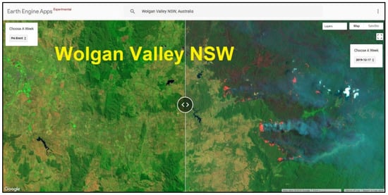
Figure 1. An overview of the Forest Fire web applications in Wolgan Valley, NSW, Australia.

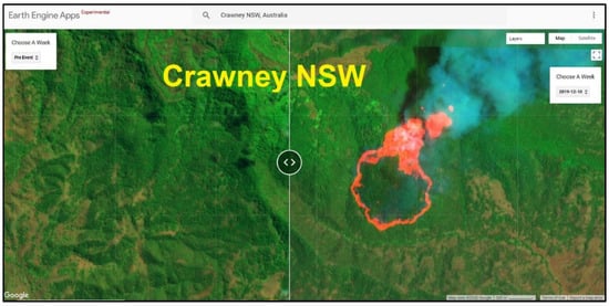
Figure 2. An example from the web app for a forest fire in Crawney, NSW, Australia.

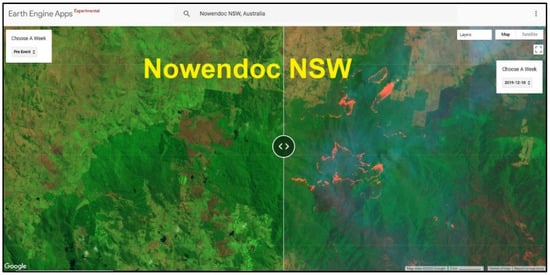
Figure 3. An example of the web app for visualizing forest fires in Nowendoc, NSW, Australia.

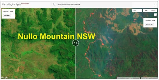
Figure 4. An example of the Forest Fire web app in Nullo Mountains, NSW, Australia.

Among all, Wolgan valley was taken as a study area from the most severely affected region, as shown by the web app.

2. Rainfall and Temperature Variation

Due to the warming climate, precipitation patterns and moisture levels change, leading to more dryness. The cooler air enhances the evaporation, leaving the soil drier by the atmosphere. Prolonged dry conditions are one of the driving factors behind forest fires. Dryness and high-temperature conditions cause the fire to occur frequently and exacerbate the length and severity of fires.

The annual rainfall time series analysis from 1981 to 2019 for Wolgan Valley was analyzed using the satellite-derived CHIRPS datasets in GEE (Figure 5). The region showed a decreasing trend (although insignificant) with a slope of −2.5. However, for 2019, the region received an annual rainfall of 596 mm, which is approximately 30% lower than the mean annual rainfall of 825 mm of the study area, which could be a major reason for the occurrence and enlargement of the forest fire. The Mann–Kendall Trend Test was also performed in order to obtain the trend behavior of the series; the test was performed based on yearly and yearly moving average. The test result is shown below in Table 1.

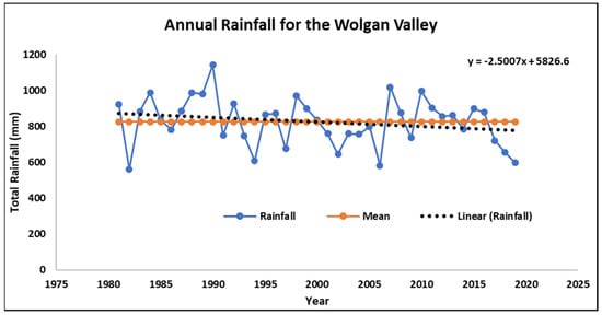
Figure 5. Annual rainfall time series from 1981–2019 for Wolgan Valley estimated from CHIRPS datasets in GEE.

Table 1. Trend analysis of CHIRPS rainfall data using Mann–Kendall moving average method.

Time Period	Trend	h	p	z	Tau	s	var_s	Slope	Intercept
Yearly	no trend	FALSE	0.110313	−1.59679	−0.17949	−133	6833.667	−0.55886	48.80874
2-yearly moving average	no trend	FALSE	0.056014	−1.91093	−0.21764	−153	6327	−0.48733	48.69761
3-yearly moving average	decreasing	TRUE	0.008567	−2.62886	−0.3033	−202	5846	−0.56612	53.42137
4-yearly moving average	decreasing	TRUE	0.001132	−3.25539	−0.38095	−240	5390	−0.66736	58.51139
5-yearly moving average	decreasing	TRUE	0.000222	−3.69237	−0.43866	−261	4958.333	−0.72488	61.15642

As shown in Table 1, the time series shows no trend when yearly data are considered, but it starts showing the decreasing trend as we move for a more realistic approach of moving average in the test. All parameters obtained by performing the Mann–Kendall trend test are shown in Table 1.

The mean annual land surface temperature (LST) time series analysis during 2001 to 2019 for Wolgan Valley was performed using the satellite derived MOD11A1.006 Terra datasets in GEE (Figure 6), which found that the region showed an increasing trend with a slope of 0.0236. Moreover, for the year of 2019, the region experienced the mean annual LST of 23.7 °C, which is approximately 8% higher than the mean annual LST of 21.9 °C. The increase in temperature has a drying effect on the flora that could be one of the reasons for the forest fire events in the region.

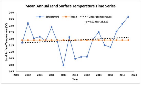
Figure 6. Annual mean land surface temperature (LST) from 2001–2019 for Wolgan Valley estimated from MODIS LST product datasets in GEE.

3. Burnt Area Estimation

The altitude for the bounding box ranges from 47 to 1599 m and is situated in the east of New South Wales. By analyzing the periodic increase in the geospatial boundary of burnt regions, we found it was 21 sq. km in October 2019, which increased to 912 sq. km in November 2019 primarily in the eastern region; later in December 2019, it further increased to 6731 sq. km with the growth in the east, north, and south directions (refer to Figure 7). So, it could be easily determined that the region suffered a severe overall increase of about 6710 sq. km within two months of the forest fire.

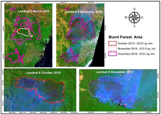
Figure 7. Map displaying the burned area footprints as estimated from visual interpretation.

The NBR multitemporal difference, i.e., due to their ease of application, the dNBR index has recently become the standard for fire intensity metrics using Landsat satellite data, as they typically provide a broad spectral range that can be accomplished between SWIR and NIR bands. The NBR pre-, NBR postestimation allows for the evaluation of change detection by multiple passes of thorough observation. From Equation (1), NBRpre and NBRpost values for the processed satellite imageries were observed. Key and Benson, (2006) who created the NBR, conceptualized the data-slicing index and suggested that the theoretical range spans from −1.0 to 1.0. An NBR near “0” means that clouds, grasses, exposed soil, or rocky outcrops can occur, and if pixels have a negative NBR, this implies extreme water stress on plants and the negative trace of a fire ^[1]. Thus, it is important to note that recent fire results usually vary from “0” to strongly negative. The dNBR (Equation (2)) combines multitemporal datasets of the NBR in one gradient, so the dNBR has a theoretical range from −2 to +2. Positive dNBR values indicate a reduction in vegetation, while negative values are a rise in vegetation cover ^[2]^[3]^[4].

Table 2 shows NBR data from the Landsat-8 image estimation for March, October, November, and December 2019. Concerning the NBR data for March 2019, it was found that pixel values ranged between −0.68 and +1.0; for October, the values ranged between −0.77 to 1; for November 2019, values ranged from −0.86 to +1.0, while the NBR data of December 2019 was found between −0.87 and +0.88.

Table 2. Theoretical and obtained bands, considering the pixels of Wolgan Valley, NSW NBR indices.

Month	Theoretical Range	NBR
Mar-19	[−1 to 1]	[−0.68 to +1]
Oct-19	[−1 to 1]	[−0.77 to +1]
Nov-19	[−1 to 1]	[−0.86 to +1]
Dec-19	[−1 to 1]	[−0.87 to +0.88]

The dNBR index for the severity groups was obtained using Equation (2). As such, Figure 8 shows the severity class for the fire burning in Wolgan Valley in the images used in this analysis. It is important to emphasize that the results of intensity display differences within the same burned area ^[5] and that determination and fire distribution perimeter, as well as the intensity within the fire, are useful for unit management managers seeking to grasp fire impacts on forests, such as the recovery of vegetation and postfire sequence for example ^[6]^[4].

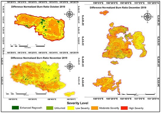
Figure 8. The dNBR indices for the identification of the severity level of the burnt area for Wolgan Valley, NSW.

The severity levels (Table 3) were used to classify the severity of indices. Moreover, we used a five-layer configuration, which has proven useful in several aspects. The dNBR value classes can differ between paired scenes. Values below −0.1 or greater than +0.66 may also exist, which may not be classified as burned. Alternatively, they are disguised as phenomena caused by lack of monitoring, clouds, or other causes not linked to actual ground cover variations.

Table 3. Severity levels and dNBR interval.

Severity Level	dNBR Range
Enhanced Regrowth	[>−0.1]
Unburned	[−0.1 to +0.1]
Low Severity	[+0.1 to +0.27]
Moderate Severity	[+0.27 to +0.66]
High Severity	[>+0.66]

The first level of severity reflects areas in which vegetation is present and can identify vegetation patches for postfire productivity. They occur almost entirely in vegetation where dNBR can be strongly negative, suggesting areas of improved after-fire efficiency (postfire NBR is much higher than pre-fire). Regular unburned pixels are located below zero. The last three stages include all other burned areas of which dNBR is explicitly constructive (postfire NBR is much less than pre-fire), including what is known as burned recently.

4. Validation

To validate the derived output of the burned area, the fire footprint for October and December 2019 were compared spatially with MCD64A1.006 MODIS Monthly Burned Area product obtained from GEE at 500 m-resolution as shown in Figure 9. On spatial interpretation, it was seen that the MODIS product overpredicted the burnt area derived from visual interpretation estimates for October and November. For October, MODIS product estimated the area to be 58 sq. km while, from Landsat-8 OLI visual interpretation, the area obtained was 22 sq. km. For December, MODIS product estimated the area to be 6205 sq. km while, from visual interpretation, the area obtained was 6731 sq. km. It could be stated that the visually interpreted region overlaps with the MODIS-derived burned area region. However, this variability could be due to the difference in their spatial resolution.

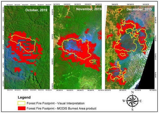
Figure 9. Forest fire footprints obtained by visual interpretation of Landsat-8 OLI and MODIS burned area products.

5. Impact on Air Pollution Due to the Forest Fire

A significant fire event recently took place in the woods of Australia from October to December 2019. A total of 5,595,739 hectares have been burned, and 2475 houses and 25 lives have been lost in 10,520 bushfires in NSW. These incidents further resulted in heavy pollution, in the form of CO and NO, in the vicinity of the event. For comparison, the air pollutants datasets were fetched for pre-fire and during-fire events.

It was found that the actual (satellite-based) mean spatial distribution of Carbon Monoxides Column Number Densities (COCND) (Figure 10) increased from 0.0177 mol/sq. m. to 0.066 mol/sq. m. during March–December 2019 with 272% change. Further, the periodic observation exhibits that the minimum and maximum COCND were 0.014 and 0.021 mol/sq. m, respectively, in March 2019, which increased to 0.022 and 0.035 mol/sq. m, respectively, in October 2019 with a 47% increase. In November 2019, it increased to a minimum and maximum value of 0.021 and 0.11 mol/sq. m, respectively, with 23% successive amplification mostly in the eastern direction. Later, in December 2019, the densities enlarged to a minimum and maximum value of 0.029 and 0.15 mol/sq. m, respectively, with 103% incremental increase in almost every direction. The stats obtained for the COCND are shown in Figure 11.

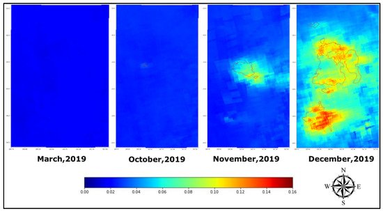
Figure 10. Maps showing the variation of COCND during the event of forest fire.

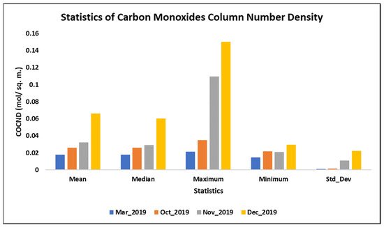
Figure 11. Statistics of COCND variation for the forest fire event.

The obtained result could also be visualized from the histogram (Figure 12a) and violin graph (Figure 12b) of the COCND images for March, October, November, and December 2019. It is found that most of the pixel counts lie close to the value of 0.01 mol/sq. m for March; for the October month, it shifts towards 0.025 mol/sq. m. For November, the pixel spans with max counts close to 0.03 mol/sq. m and, finally, for December 2019, the pixels become very distributed with maximum counts close to the value of 0.05 mol/sq. m.

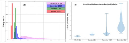
Figure 12. (a) Histogram and (b) Violin plot obtained for the COCND values for the forest fire incident.

Similarly, the overall trend of mean Nitrogen Oxides Column Number Densities (NOCND) (Figure 13), for the forest area was found to increase from 0.0000287 mol/sq. m to 0.0000416 mol/sq. m during March–December 2019 with 45% change. It was observed that the minimum and maximum NOCND were 0.0000027 and 0.0002496 mol/sq. m, respectively, in March 2019, which increased to 0.0000041 and 0.0002627 mol/sq. m, respectively, in October 2019 with a 10% increase. In November 2019, it decreased to a minimum and maximum 0.0000033 and 0.0002478 mol/sq. m, respectively, with a 6% decrease. However, again in December 2019, the densities increased to a minimum and maximum value of 0.0000033 and 0.0004636 mol/sq. m, respectively, with 40% incremental increase. The stats obtained for the NOCND is shown in Figure 14.

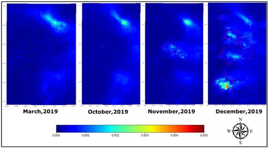
Figure 13. Maps showing the variation of NOCND during the event of forest fire.

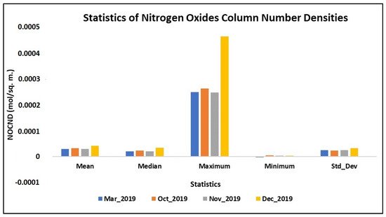
Figure 14. Statistics of NOCND variation for the forest fire event.

The obtained result could also be visualized from the histogram (Figure 15a) and violin graph (Figure 15b) of the NOCND images for March, October, November, and December 2019. It is found that most of the pixel counts lie close to the value of 0.0000116 mol/sq. m for March and, for October, it shifts towards 0.0000155 mol/sq. m. For November, the pixel value reduces to 0.000012 mol/sq. m and, finally, for December 2019, the pixels get distributed with maximum counts close to the value of 0.00002 mol/sq. m.

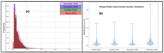
Figure 15. (a) Histogram and (b) Violin plot obtained for the NOCND values for the forest fire incident.

The increase in CO is attributed to incomplete biomass combustion. NO emissions are due to the high nitrogen content of biomass and new leaves. The analysis reveals that forest fire does not just affect the ecosystem in which it occurs, but also has effects on the surrounding regions.

References

Key, C.H.; Benson, N.C. Landscape Assessment: Ground Measure of Severity, the Composite Burn Index; and Remote Sensing of Severity, the Normalized Burn Ratio. 2006. Available online: http://pubs.er.usgs.gov/publication/2002085 (accessed on 20 August 2021).
Miller, J.D.; Thode, A.E. Quantifying burn severity in a heterogeneous landscape with a relative version of the delta Normalized Burn Ratio (dNBR). Remote Sens. Environ. 2007, 109, 66–80.
Soverel, N.O.; Perrakis, D.D.; Coops, N.C. Estimating burn severity from Landsat dNBR and RdNBR indices across western Canada. Remote Sens. Environ. 2010, 114, 1896–1909.
Dos Santos, S.M.B.; Bento-Gonçalves, A.; Franca-Rocha, W.; Baptista, G. Assessment of burned forest area severity and postfire regrowth in chapada diamantina national park (Bahia, Brazil) using dnbr and rdnbr spectral indices. Geosciences 2020, 10, 106.
Roy, D.P.; Boschetti, L.; Trigg, S.N. Remote sensing of fire severity: Assessing the performance of the normalized burn ratio. IEEE Geosci. Remote Sens. Lett. 2006, 3, 112–116.
Escuin, S.; Navarro, R.; Fernández, P. Fire severity assessment by using NBR (Normalized Burn Ratio) and NDVI (Normalized Difference Vegetation Index) derived from LANDSAT TM/ETM images. Int. J. Remote Sens. 2007, 29, 1053–1073.

© Text is available under the terms and conditions of the Creative Commons Attribution (CC BY) license; additional terms may apply. By using this site, you agree to the Terms and Conditions and Privacy Policy.

Upload a video for this entry

Information

Subjects: Environmental Sciences; Engineering, Geological; Remote Sensing

Contributor MDPI registered users' name will be linked to their SciProfiles pages. To register with us, please refer to https://encyclopedia.pub/register :

Suraj Singh

View Times: 501

Entry Collection: Environmental Sciences

Update Date: 28 Dec 2021

Table of Contents

Video Upload Options

Confirm