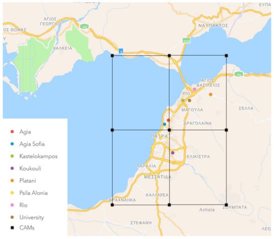
Air pollution is a global pivotal issue in the fields of health and environment, affecting at the same time both the economy and social life. Expediting industrialization and urbanization triggered an increase in cardiovascular and lung diseases, attributable to air pollution ^[1]. Airborne particles with a diameter of 10 μm or less are included in air pollutants with adverse effects on public health, especially in urban areas. Particulate matter (PM) consists of a complex mixture of particles with major components sulfate, nitrates, ammonia, sodium chloride, black carbon, mineral dust and water ^[2]. Both coarse particulate matter (PM10) and fine particles (PM2.5), due to their diminutive size, can penetrate deeply into the respiratory system, causing serious chronic health problems including airway irritation, asthma, irregular heart rate, abnormal lung function ^[3][4]. Long-term exposure to high levels of PM is quantitatively associated with increased mortality and lung cancer ^[2]. Fine particles are small and light, which allows them to remain in the atmosphere for longer periods of time; they also have been associated with a 4 to 8% increase in the burden of cardiopulmonary diseases ^[5]. The sources of particulate matter (PM), in their majority, are anthropogenic, with the natural sources constituting a small portion of the total concentration ^[6]. Consequently, particle pollution in urban areas is significantly higher due to the accumulation of primary sources of PM2.5 and PM10, including industrial and vehicle emissions, fuel oils and indoor activities ^[7].

In this context, to protect the quality of life from the devastating effects of elevated pollutant concentrations, the designing of effective strategies and the redefining of limits concerning emissions produced by industrial sources and vehicle traffic are considered imperative. Air quality forecasting is a preliminary step in establishing abatement measures leading to the prevention and the control of air pollution. Accurate and constant estimation of air pollutant concentrations ensures regular and direct information flow, facilitating reasonable decision-making and direct execution of the action plan. In this respect, much effort has been made for the development of air quality forecasting models to provide a scientifically based planning ^[8]. Achieving early warning has the potential to limit environmental pollution, determining additional control requirements, and developing new technologies and practical applications to reduce the levels of air pollutants. In addition, using all the information provided and with thorough directions given by the Civil Protection, vulnerable groups can limit their outdoor activities on high-pollution days ^[9].

The Copernicus Atmosphere Monitoring Service (CAMS) ^[10] of the European Center for Medium-Range Weather Forecasts (ECMWF) ^[11], which monitors the atmospheric composition, provides reliable and quality-controlled information for immediate use. This open-access platform delivers forecasts about common air pollutants on a global scale. The air quality forecasts are the median ensemble from the outputs of nine air quality models and are produced for the next four days. CAMS simulates the dilution and dispersion of air pollutants that affect the atmosphere, contributing crucially to the comprehension of its processes. However, uncertainties introduced by the input parameters, the initial and boundary conditions, constitute defects ^[12][13][14]. Further, the coarse resolution of CAMS limits its applicability mostly to non-urban areas.

Statistical methods are often applied into the forecasts of a numerical model to improve its skill. Various post-processing techniques (including analog-based, AI-based, SL-based) forecasting essentially the uncertainty involved in AQ models manage to enhance their forecast skill ^{[15][16][17][18]}.

Analog Ensemble is a technique that produces deterministic and probabilistic air pollution forecasts by using deterministic numerical weather predictions (NWP) and their contemporary observations, combined with a statistical post-processing method. It was proposed by Delle Monache et al. ^[19] and has been successfully generating predictions for air pollutants ^[20][21]. Likewise, in the analog-based methods, the prediction is based on previous times, which present similar conditions to the current state of the atmosphere ^[22]. The uncertainty of the current forecast is estimated, considering the corresponding uncertainties of past similar forecasts.

Deep learning is a widespread method in air pollution prediction ^[23][24] because of its potential in handling non-linear data structure and multivariate time series analysis problems. The vast amount of data used in air quality problems, generated by various sources, can be analyzed effectively by artificial neural networks, suitable for big data processing and tackling complex problems. The complex issue of air pollution prediction demands sequential data, covering a long time range, and issued from the dynamic system of the atmosphere. To deal with problems of the same nature, long short-term memory networks (LSTMs) were proposed ^[25]. LSTM networks generate deterministic forecasts of particulate matter, as a function of input lagged variables, trying to find patterns recognition in the past.

Data-driven models can generate forecasts on the basis of reliable measurements. Numerous sensor models are used to monitor air quality in cities, with the low-cost sensors gaining popularity both for their potential to be installed in dense distribution, and for their affordable operational cost. Their reliability is in dispute when compared with (high-quality sensors) grade monitoring stations due to the data variability or lower accuracy. However, calibrating them with the appropriate techniques can generate reliable data in increased spatial coverage ^[26][27][28].

In this study, we evaluate the CAMS PM forecasts at a local scale against in-situ measurements, spanning 2 years, obtained from a dense network of calibrated low-cost air pollution stations located in an urban coastal Mediterranean city in Greece. Then, we apply two essentially different statistical approaches into the operational CAMS forecasts to investigate their predictive capacity to accurately map the pollution pattern at a local scale for different types of stations (urban, suburban, rural). Specifically, AnEn and LSTM methods are trained with the 4-day-ahead operational forecasts of PM10 and PM2.5 from CAMS as well as open data from ground-based observations for 2018 and tested with the corresponding datasets of 2019.

2. Observed PM Concentrations

3. CAMS Evaluation

4. Development of AnEn and LSTM Models

LSTM and AnEn methods are employed to produce PM10 and PM2.5 forecasts for the next 90 h at six-hour increments, for the eight air quality monitoring stations located in the urban area of Patras. The datasets of all the stations are separated into two parts, one for training the models (2018) and the other for evaluating them (2019). In this section, we present the implemented configuration of each algorithm issued during the training phase.

4.1. AnΕn

Given a forecast, the AnEn algorithm searches similar past forecasts in the training dataset, as described in Section 2.2.1. The selection of the number of analogs and the combination of predictors contribute significantly to the optimal configuration of the AnEn method. Those factors are determined by the leave-one-out cross-validation method in the training dataset (2018) applied for each day. PM10 and PM2.5 are the target variables. The predictor variables for PM10 (PM2.5) are four: the same variable provided from the CAMS forecast and three auxiliary variables, namely, the CAMS forecast of PM2.5 (PM10), the Julian day and the day of week. Seven combinations are produced by the set of the three auxiliary variables, which, with the addition of the AnEn that hasn’t any auxiliary variable, produce a total of eight combinations. For each station, the number of analogs and the variable combination yielding the lowest RMSE between the observed values and the analog ensemble predictions in the train period are identified. The same configuration will be applied in the next section, in the ‘blind’ dataset of the validation period.

Table 2 displays the optimum configuration per station, i.e., the number of analogs and the combination of predictor variables yielding the minimum RMSE. At most stations, more than 20 analogs are needed to derive the analog forecast for PM2.5 while fewer members (on average 6 less) are required for PM10 forecasts. In producing PM10 predictions, PM2.5 is used from all stations while the contrary is generally not true, occurring only at 25% of the stations. For both pollutants, AnEn utilizes as input the Julian day at most stations (seven out of the eight) while WDAY was found important at 2–3 stations only. Hence, the AnEn PM10 forecast relies mostly on three inputs (CAMS forecasts of PM10 and PM2.5, Julian day) while the AnEn PM2.5 forecast has two dominant inputs (CAMS forecast of PM2.5, Julian day). This partly explains the need for fewer analogs for PM10. Adjusting weights to the predictors does not led to better results because they are proven statistically insignificant.

4.2. LSTM

Achieving the best performance for the LSTM model is a complex and time-consuming procedure. It is not enough to optimize the hyperparameters of the model; the best combination of them should also be found. In order to construct the architecture of the LSTM network, hyperparameters like the number of hidden layers and nodes in each layer are used, while epoch and batch size, optimizer, loss and activation function should also be employed. A range of values is tested for adjusting each parameter. Through a grid search, numerous trials with all the possible parameter combinations are conducted to result in the final network. As input variables, the same are used as those of AnEn, i.e., observations and CAMS forecasts of PM10 and PM2.5, the Julian day and the day of week. The data for 2018 of each station are divided into groups of four days, using the first three days of each group as a training set and the fourth day as a validation set to tune the hyperparameters of the model.

The dataset needs preparation before introducing it to the LSTM network, including normalizing the input variables with a range of 0–1 and transforming it suitably for a supervised learning problem. Investigating the correlation between the current target value and its own historical lagged values through the partial autocorrelation (PACF) function, the higher correlation occurred four steps back (t-24 h). Therefore, the LSTM network is trained with a time lag of four timesteps. Using as input the prior four timesteps of predictors (at time t-24 h), the LSTM model is learning from them to produce PM forecasts for each forecast lead time for the next four days.

Based on trial experiment runs, one LSTM layer is proven suitable for the network to avoid overfitting, Although the number of 100 units in the hidden layer seems to be appropriate for all stations, a different network size s tested to achieve the best result for each station. As a concern, the activation of this layer is selected between the functions of relu, sigmoid, softmax and tanh, with the sigmoid function yielding to the least Mean Square Error. After the LSTM layer, two dense layers are added; the first is a fully connected layer with 50 units that works efficiently to connect the neurons to each layer, with the second dense layer acting as the output layer. The output of the model is one-dimensional and utilizes sigmoid activation to produce better forecasts. The model is trained using the Adam gradient-based optimization technique. The Adam optimizer compared with two other stochastic gradient descent algorithms, Stochastic Gradient Descent (SGD) and RMSProp, achieves the minimum error with the lesser number of epochs. After the selection of the optimizer, the number of epochs and batch size are determined, 50 and 76, respectively. For the validation loss, the function must be minimized through optimization, where common choices are the RMSE and MAE. In this case, the RMSE is proven to be a better option. Many of the mentioned results are in accordance with the findings reported in pertinent studies on air pollution forecasting with LSTM models ^[29][30][31].

5. AnEn & LSTM Forecast Verification (Validation Phazse)

In this section, the optimal configuration of AnEn and LSTM identified during the training phase in the year 2018 (Section 3.3) is applied to the 2019 dataset to evaluate their forecast skill. The verification is carried out for each station separately, covering different forecast lead times, seasons and extreme levels. Verification of CAMS forecasts pin-pointed to the station locations are also used for comparison.

5.1. Time Series

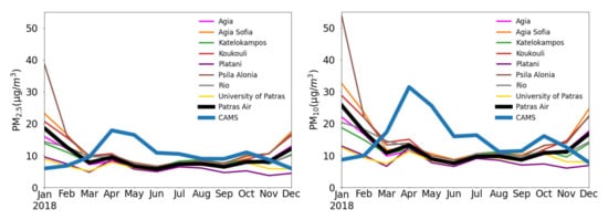
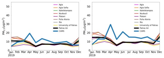
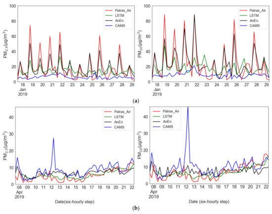
Concurrent time series of PM predictions by CAMS, LSTM and AnEn techniques against ground-level observations are produced at six-hour increments for all sites of the study. Figure 3 illustrates the time-series plots of two stations of different types, an urban traffic station (Psila Alonia) and a suburban background station (University of Patras), for a two-week period of January and April 2019, respectively. Those months are selected because, as seen earlier, of the deviation between observations and CAMS peaks during those months. As far as the urban traffic station is concerned (Figure 3a), despite the tendency of CAMS to underestimate PM concentrations conspicuously in January, the AnEn is drastic in correcting the CAMS forecasts towards the magnitude and variability of the measured values. The LSTM captures the variations of the measured values; however, it underestimates the peaks, making it inferior to the AnEn in this type of station. Regarding the background suburban station (Figure 3b), the CAMS model produces quite overestimated forecasts during April. The application of the AnEn in the CAMS forecasts limits to a large extent their distance from the observations. The LSTM, integrating antecedent useful information to the next output, accomplishes a good performance even though it tends to overestimate the minimum. In summary, both the AnEn and the LSTM demonstrate a significant potential to correct the magnitude and phasing of CAMS PM2.5 and PM10 predictions, with AnEn displaying higher forecast skill at the occasional observed extreme PM concentrations.

5.2. Degradation of Forecast Skill

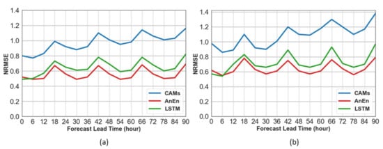
The verification of the daily cycle of the models has been carried out for horizons up to 90 h ahead, at the eight air quality monitoring stations. Figure 4 displays the normalized RMSE as a function of the forecast lead time from hour 0 to 90 for the PM2.5 and PM10 levels. The improvements over CAMS are significant at all stations for each forecast lead time. The AnEn generates better results than the LSTM method. The peak error in both approaches is observed at 18 h UTC due to the elevated levels of PM at the specific evening rush time. Moreover, the degradation of the forecast skill as the forecast interval increases is milder for the corrected schemes, being slowest for AnEn (0.015 increase in NRMSE per forecast day) compared to LSTM (0.043 per day) and CAMS (0.079 per day).

5.3. Error Indices

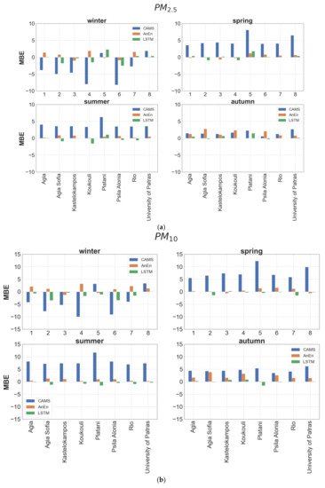
Typical error metrics, such as MBE and RMSE, are calculated at each monitoring station in annual, seasonal and monthly temporal scales to gain insight on the forecast skill of each model. On an annual scale, CAMS shows positive bias for both pollutants, with the MBE of PM10 being roughly double compared to PM2.5 (Table 3). As illustrated in Figure 5, the annual overestimation from CAMs is found for all seasons except for winter, when quite underestimated forecasts are distinguishable. The annual biases of both approaches are smaller than 1 μg/m⁻³ in absolute terms when aggregated over all stations, being reduced compared to CAMS by a factor of at least 3 (Table 3). The AnEn technique reduces the bias of CAMS forecasts by approximately 65%, in absolute terms. On the annual scale, it generates predictions with a slight overestimation, in the range 0.1 to 1.1 μg/m⁻³ for PM2.5 and 0.2 to 1.7 μg/m⁻³ for PM10. The bias reduction is consistent across all seasons. In contrast to AnEn, the LSTM model exhibits a minor underestimation tendency ranging from −0.9 to 1.7 μg/m⁻³ for PM2.5 and −1.4 to 0.2 μg/m⁻³ for PM10, which demonstrates slightly underestimated concentrations with small negative MBE values.

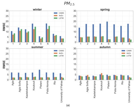
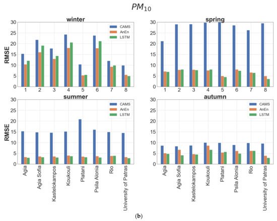
The performance of each model is also evaluated using RMSE, a widely used reliability factor where errors of different signs do not compensate as in the case of MBE. As can be inferred from Table 4, neither method is clearly superior. Both models show a gross annual RMSE value (averaged over all stations) lower by approximately 50% for PM2.5 and 60% for PM10 with respect to CAMS. The best performance (~75% RMSE improvement) for both models is met at the suburban background stations (University of Patras, Platani) and the worst (~50% RMSE improvement) is noticed at the urban traffic stations (Koukouli, Psila Alonia). AnEn prevails over the LSTM method in urban traffic stations (high PM levels) while the opposite is true at the background stations. According to the seasonal values of RMSE at each station, the AnEn attains better results than LSTM during winter (Figure 6). The largest improvement of AnEn over CAMS forecasts is observed in spring and summer and the minimum in autumn. Generally, in terms of RMSE, AnEn is proven more efficient for predicting periods with high particulate air pollution levels, whereas the LSTM is marginally more successful, in seasons with moderate emissions.

References

- Brauer, M.; Amann, M.; Burnett, R.T.; Cohen, A.; Dentener, F.; Ezzati, M.; Henderson, S.B.; Krzyzanowski, M.; Martin, R.V.; Van Dingenen, R.; et al. Exposure assessment for estimation of the global burden of disease attributable to outdoor air pollution. Env. Sci. Technol. 2012, 46, 652–660.
- WHO. Review of Evidence on Health Aspects of Air Pollution—REVIHAAP Project: Technical Report; WHO: Copenhagen, Denmark, 2013; p. 302.
- Lelieveld, J.; Evans, J.S.; Fnais, M.; Giannadaki, D.; Pozzer, A. The contribution of outdoor air pollution sources to premature mortality on a global scale. Nature 2015, 525, 367–371.
- Pope, C.A.; Dockery, D.W.; Schwartz, J. Review of Epidemiological Evidence of Health Effects of Particulate Air Pollution. Inhal. Toxicol. 1995, 7, 1–18.
- Pope III, C.A.; Burnett, R.T.; Thun, M.J.; Calle, E.E.; Krewski, D.; Ito, K.; Thurston, G.D. Lung Cancer, Cardiopulmonary Mortality, and Long-term Exposure to Fine Particulate Air Pollution. JAMA 2002, 287, 1132–1141.
- Urch, B.; Brook, J.R.; Wasserstein, D.; Brook, R.D.; Rajagopalan, S.; Corey, P.; Silverman, F. Relative Contributions of PM2.5 Chemical Constituents to Acute Arterial Vasoconstriction in Humans. Inhal. Toxicol. 2014, 16, 345–352.
- EEA. Air Quality in Europe—2019 Report; EEA Report No 10/2019; European Environment Agency: Copenhagen, Danmark, 2019; Available online: (accessed on 20 January 2021).
- Li, L.; Zhang, J.H.; Qiu, W.Y.; Wang, J.; Fang, Y. An Ensemble Spatiotemporal Model for Predicting PM2.5 Concentrations. Int. J. Environ. Res. Public Health 2017, 14, 549.
- Salnikov, V.G.; Karatayev, M.A. Impact of air pollution on human health: Focusing on Rudnyi Altay industrial area. Am. J. Environ. Sci. 2011, 7, 286–294.
- CAMS. Available online: (accessed on 28 December 2020).
- ECMWF. Available online: (accessed on 28 December 2020).
- Kalnay, E. Atmospheric Modelling, Data Assimilation and Predictability; Cambridge University Press: Cambridge, UK, 2003; p. 341.
- Kioutsioukis, I.; Melas, D.; Zerefos, C.; Ziomas, I. Efficient Sensitivity Computations in 3D Air Quality Models. Comput. Phys. Commun. 2005, 167, 23–33.
- Zhang, Y.; Seigneur, C.; Bocquet, M.; Mallet, V.; Baklanov, A. Real-Time Air Quality Forecasting, Part II: State of the Science, Current Research Needs, and Future Prospects. Atmos. Environ. 2012, 60, 656–676.
- Borrego, C.; Monteiro, A.; Pay, M.T.; Ribeiro, I.; Miranda, A.I.; Basart, S.; Baldasano, J.M. How bias-correction can improve air quality forecasts over Portugal. Atmos. Environ. 2011, 45, 6629–6641.
- Delle Monache, L.; Nipen, T.; Liu, Y.; Roux, G.; Stull, R. Kalman filter and analog schemes to postprocess numerical weather predictions. Mon. Weather Rev. 2011, 139, 3554–3570.
- Kioutsioukis, I.; Galmarini, S. De praeceptis ferendis: Good practice in multi-model ensembles. Atmos. Chem. Phys. 2014, 14, 11791–11815.
- Kioutsioukis, I.; Im, U.; Solazzo, E.; Bianconi, R.; Badia, A.; Balzarini, A.; Baró, R.; Bellasio, R.; Brunner, D.; Chemel, C.; et al. Insights into the deterministic skill of air quality ensembles from the analysis of AQMEII data. Atmos. Chem. Phys. 2016, 16, 15629–15652.
- Delle Monache, L.; Eckel, F.A.; Rife, D.L.; Nagarajan, B.; Searight, K. Probabilistic weather prediction with an analog ensemble. Mon. Weather Rev. 2013, 141, 141,3498–516.
- Delle Monache, L.; Alessandrini, S.; Djalalova, I.; Wilczak, J.; Knievel, J.C.; Kumar, R. Improving Air Quality Predictions over the United States with an Analog Ensemble. Weather Forecast 2020, 35, 2145–2162.
- Djalalova, I.; Delle Monache, L.; Wilczak, J. PM2.5 analog forecast and Kalman filtering post-processing for the Community Multiscale Air Quality (CMAQ) model. Atmos. Environ. 2015, 119, 431–442.
- Hamill, T.M.; Whitaker, J.S. Probabilistic quantitative precipitation forecasts based on reforecast analogs: Theory and application. Mon. Weather Rev. 2006, 134, 3209–3229.
- Qi, Z.; Wang, T.; Song, G.; Hu, W.; Li, X.; Zhang, Z. Deep air learning: Interpolation, prediction, and feature analysis of fine-grained air quality. IEEE Trans. Knowl. Data Eng. 2018, 30, 2285–2297.
- Zhang, Y.; Wang, Y.; Gao, M.; Ma, Q.; Zhao, J.; Zhang, R.; Wang, Q.; Huang, L. A Predictive Data Feature Exploration-Based Air Quality Prediction Approach. IEEE Access 2019, 7, 30732–30743.
- Hochreiter, S.; Schmidhuber, J. Long Short-Term Memory. J. Neural. Comput. 1997, 9, 1735–1780.
- Feenstra, B.; Papapostolou, V.; Hasheminassab, S.; Zhang, H.; Der Boghossian, B.; Cocker, D.; Polidori, A. Performance evaluation of twelve low-cost PM2.5 sensors at an ambient air monitoring site. Atmos. Environ. 2019, 216, 116946.
- Kosmopoulos, G.; Salamalikis, V.; Pandis, S.N.; Yannopoulos, P.; Bloutsos, A.A.; Kazantzidis, A. Low-cost sensors for measuring airborne particulate matter Field evaluation and calibration at a South-Eastern European site. Sci. Total Environ. 2020, 748, 141396.
- Pope, F.D.; Gatari, M.; Ng’ang’a, D.; Poynter, A.; Blake, R. Airborne particulate matter monitoring in Kenya using calibrated low-cost sensors. Atmos. Chem. Phys. 2018, 18, 15403–15418.
- Athira, V.; Geetha, P.; Vinayakumar, R.; Soman, K. Deepairnet: Applying recurrent networks for air quality prediction. Procedia Comput. Sci. 2008, 132, 1394–1403.
- Chaudhary, V.; Deshbhratar, A.; Kumar, V.; Paul, D. Time Series Based LSTM Model to Predict Air Pollutant’s Concentration for Prominent Cities In India. 2018. Available online: (accessed on 20 January 2021).
- Kingma, D.P.; Ba, J.A. A method for stochastic optimization. arXiv 2014, arXiv:1412.6980.