Electrical Source Imaging

Version	Summary	Created by	Modification	Content Size	Created at	Operation
1		Ioannis Kakkos	+ 2658 word(s)	2658	2021-06-29 11:37:21	\|
2	update layout and reference	Rita Xu	Meta information modification	2658	2021-07-13 07:56:01	\|

This entry is adapted from the peer-reviewed paper 10.3390/signals2030024

Electrical Source Imaging (ESI) is an imaging technique utilized to localize the activated brain regions by incorporating temporal and spatial components from electroencephalogram (EEG) signals.

EEG source imaging source localization applications challenges

1. Introduction

Electrical Source Imaging (ESI) is an imaging technique utilized to localize the activated brain regions by incorporating temporal and spatial components from electroencephalogram (EEG) signals. Although this imaging method provides fine temporal resolution compared to other imaging methods, such as the functional magnetic resonance imaging (fMRI), the number of electrodes used to record the brain electrical potentials is significantly smaller than the number of activated neurons, rendering EEG source localization an ill-posed problem. To determine the generating source of the brain’s electrical activity, the scalp potentials (i.e., the potentials created by the synchronous activation of pyramidal neurons in the brain ^[1], which are propagated through the different tissues that compose the head) are recorded by an array of surface electrodes. Then, an estimation of the signals’ origin is calculated through Poisson’s equation ^[2]. Poisson’s equation is directly derived from Maxwell’s equations, given that the head tissues have the permeability of free space, while the localization of the activated regions within the brain is commonly referred to in the literature as the inverse problem. On the contrary, computing the scalp potentials from a given source (a prerequisite to calculate inverse solutions) is designated as the EEG forward problem. As such, given that Poisson’s equation highly depends on the accurate values of the electrical and geometrical properties (thickness, conductivity, etc.) of the head tissues (scalp, skull, cerebrospinal fluid (CSF), brain cavities, etc.), it is evident that a precise head model is critical to solve the forward problem correctly. To address this, anatomical information can be provided by magnetic resonance imaging (MRI). Nevertheless, it is extremely difficult to obtain head MRI in a subject-specific fashion. Thus, a large number of studies rely on template anatomical information ^[3]^[4]^[5]. Having a proper head model also facilitates the correct electrode positioning, since the location of each electrode varies for each individual (although to a small degree). In this context, the anatomical information as well as the corresponding electrode locations comprise the Leadfield matrix, the accurate calculation of which is closely related to the accuracy of the solutions of the inverse problem ^[6]. The EEG source localization has puzzled researchers since a vast variety of combinations of sources can produce the same signals recorded by the EEG ^[7]. This is a fundamental problem of EEG source localization, because even with a flawless head model and an excellent noiseless signal, the number of equations that can be solved is minuscule compared to the number of dipoles (source points) within the brain, leading to non-unique possible solutions. This non-uniqueness can be handled with mathematical, anatomical or neurophysical constraints about the location and the direction of dipoles ^[8]^[9]. Therefore, even if non-uniqueness is not guaranteed, these a priori assumptions are utilized, in order to reduce the computational needs for the source estimation and increase the accuracy of the solutions.

However, owing to recent advances which incorporate novel methodologies as well as the introduction of machine learning approaches in solving the inverse problem ^[10]^[11], the required time and the computational resources for the solution have been significantly reduced. Furthermore, sophisticated algorithms have diminished the localization error efficiently, estimating the location and activation of the different cortical regions ^[12]. This is evident in several applications, ranging from detecting and assisting the therapy of epilepsy, to interpreting emotions from facial expressions ^[6]^[13].

2. State-of-the-Art

In this paper, current ESI implementation approaches, trends and challenges are presented. The databases examined for the synthesis of the studies presented were—PubMed, Scopus, ScienceDirect and Google Scholar. Eligibility criteria included research works that incorporate recent advancements (published after 2015) regarding forward and inverse solutions, clinical and cognitive applications and methodological/algorithmic aspects of source imaging.

2.1. Forward Problem

To solve the EEG forward problem, three main configurations are required—(a) the head and source models (i.e., the location of the solution points in the brain), (b) the electrode alignment on the head model, and (c) the Leadfield matrix using the channel locations in relation to the anatomical information of the head model. As such, the solution’s accuracy highly depends on the efficient generation and composition of the above. The basic components and the flow of processes are shown in Figure 1.

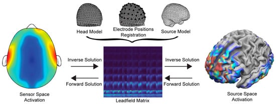
Figure 1. Information flow and basic components of the forward and inverse problems.

Regarding the creation of the head model, the integration of anatomical data has rendered earlier widely adopted spherical head models outdated ^[14]. Converting MRI images into head models is a time-consuming process with a high computational cost, and this procedure presents optimal results in terms of localization accuracy. Nevertheless, subject-specific MRI recordings are not always available, requiring the head model to be constructed through computational methods. In this regard, however, it is important to emphasize that the sophistication of the head models does not display a linear trend with ESI localization, leading to high implementation complexity (e.g., inclusion of skull spongiosa) to demand significant computational resources, with little to no significant impact in spatial accuracy ^[15]^[16].

The most common methods utilized for head-modeling are the boundary element methods (BEMs), finite difference methods (FDMs) and the finite element methods (FEMs) ^[17]^[18]^[19]^[20]. The Projective Method (PM) (that incorporates the mathematical descriptors of surfaces, such as Fourier descriptors, and dimensionality reduction methods, such as Principal Component Analysis), is also well established, albeit less common ^[21]^[22]. Of note is that for PM, in contrast with the aforementioned methods, the time required to extrude the head model and the computational resources is drastically reduced, but with lower spatial resolution ^[23].

Regarding the frequently employed algorithms, FEM and FDM provide more analytical outcomes and can tackle inhomogeneity problems, which is vital if the head model requires the modeling of anisotropic properties of white matter and the skull. On the other hand, BEM presents lower computational time and accuracy in comparison to the FEM and FDM, being unable to treat inhomogeneous and nonlinear problems.

Even though the FEM approach provides a more well-established detailed model, since it incorporates more than the three standard head tissues, its universal implementation has been hamstrung due to its computational needs and lack of open-source tools incorporating a complete FEM approach. However, the Fieldtrip–SimBio pipeline has been recently introduced, providing an integrated EEG forward problem solution, while employing an FEM-created head model ^[24]. On this premise, it should also be noted that subject-specific MRIs are not always possible to be recorded. For this reason, an averaged (standardized) volume conductor model using the ICBM 152 anatomical template and the FEM (“The New York Head”) was created, showing promising results in ESI, compared to other standardized FEM and BEM approaches ^[25]. While FEM effectiveness is shown to be comparable with analytical solutions ^[26], adverse issues could occur due to skull leakage effects (i.e., the inhomogeneity of skull thickness), which could lead the implemented model to present similar properties to a simple three-layer sphere model ^[27]. In order to overcome this inconsistency, different FEM approaches are used, deviating from the standard continuous Galerkin–FEM method (CG-FEM) by creating a mixed or discontinuous Galerkin–FEM utilizing the subtraction approach ^[28]^[29]. Evidence suggests that this solution combines the benefits from both approaches, decreasing the skull leakage effect ^[19]. Furthermore, using analytical expressions combined with the subtraction approach, the accuracy of the forward problem solution was increased compared to other numerical approaches with similar computational costs ^[30]. Increments in the precision of the EEG forward problem results have also been demonstrated by the incorporation of tissue inhomogeneity, even within the gray and white matter ^[31]. Apart from FEM, computationally efficient and accurate solutions have also been achieved with the introduction of anisotropic conductivity equations and utilization of the reciprocity theorem ^[32] on FDM head models (AFDRM-NZ) ^[33]. In this regard, anisotropic conductivity values are integrated by employing a set of surface integral equations aligning the produced solutions with the analytical results ^[34]. Of note is that the skull conductivity and, therefore, the correct modeling is a pivotal point, which, due to head abnormalities or insufficient imaging tools, can be challenging to approximate ^[35]. To address this issue, Bayesian Approximation Error (BAE) approaches displayed high efficiency in reducing the source localization error by several millimeters, enhancing spatial accuracy, which is crucial in clinical applications ^[36].

2.2. Inverse Problem

Contrary to the forward problem, the inverse problem cannot be uniquely solved if there are no a priori restrictions about the source locations ^[37]. This fact has led researchers to incorporate various mathematical constraints preceding the source estimation, thus reducing the number of possible solutions deriving from the recorded data. Such constraints are the core of many of the conventional methods used to solve the inverse problem. The inverse methods that are commonly used fall into two main categories—non-parametric (non- adaptive) and parametric (adaptive) distributed source imaging.

Although there is an extremely large number of ESI methodologies for parametric (e.g., Beamformers, Multiple Signal Classification) and non-parametric (e.g., Minimum Norm Estimate, Focal Underdetermined System Solution, Local Auto-Regressive Average) distributed source imaging methods of the inverse solution, in this paper, we focus on the most commonly employed algorithms, to highlight the progress of ESI. For an extensive review of the mathematical aspects and properties of several of these conventional methods and their variants, that are beyond the scope of this review paper, please refer to the thorough reviews ^[38]^[39].

The most frequent non-parametric algorithms employed are the minimum norm estimate (MNE) solution ^[40] and its depth-weighted variant (dw-MNE) ^[41]^[42], although several other designs take into account the same principles with modified settings and additional parameter incorporation. For instance, the low resolution electromagnetic tomography activity (LORETA) estimates the current density given by the minimum norm solution but with a more sophisticated regularization, utilizing a discrete Laplace operator that selects preferentially spread source (“smooth”) distributions, in contrast with the MNE’s identity matrix ^[43]^[44]. On the other hand, parametric distributed source imaging methods commonly include Linear Constrained Minimum Variance (LCMV) beamformers that depend on structurally related filters to provide efficient source localization irrespective of noise covariance ^[45]. Contrary to the non-parametric approaches for solving the inverse solution, LCMV beamformers isolate the signals produced by different parts of the brain using spatial filters, thus allowing the solution computations to occur independently for each solution point.

Even though conventional methods have been proven to be efficient in determining the activated brain regions, emerging technologies in the fields of Machine and Deep Learning have been recently introduced in ESI. As such, a novel method proposed for solving the inverse problem utilizes the deep recurrent neural network architecture of long-short term memory (LSTM) units in an auto-encoder framework, presenting exceptional mean localization error of less than 5 mm on single-source simulated data ^[10]. This architecture is able to model the spatio-temporal information provided by training the network to perceive the correlation between the location of the source and the EEG signals without needing a priori constrictions, normally provided manually by more conventional methods. In a similar manner, ConvDip, a convolutional neural network (CNN), has demonstrated a lower normalized mean squared error in ESI solutions compared to that of exact LORETA (eLORETA) and beamformers for a single source, utilizing a shallow CNN with one convolutional layer and two fully connected layers ^[11]. Compared to the LSTM approach, ConvDip was trained with single time-instances on simulated data but with multiple sources. This is important, since a large variety of inverse solutions, such as eLORETA and LCMV beamformer, rely on noise covariance matrices that are computed with the temporal information of EEG signals, significantly affecting the accuracy of the model if the noise is increased. Moreover, the fact that simple networks can learn the patterns of single time points and predict reasonable inverse solutions is a major point in lowering complexity and consequently computational cost. Additional ESI neural networks frameworks include a denoising AutoEncoder (DST-DAE) consisting of six layers, three encoding blocks and three decoding blocks. This method was able to directly map the EEG and magnetoencephalogram (MEG) signals to the cortical sources, reducing the localization error to less than a millimeter ^[46]. In this regard, both temporal and spatial information is utilized on synthetic data, in order to extract inverse mapping. The main advantage of this method lies in its resistance and robustness against low Signal-to-Noise ratio (SNR), resulting in efficient source estimation with excellent denoising properties. Added together, the recent advances in Machine Learning ESI estimation indicate the efficacy of the employed procedures in contrast to the traditional model-driven approaches, especially since in all of the data-driven methods, very few or no mathematical priors were used, while the need for optimizing parameters for new data is absent.

Apart from Deep Learning designs, recent studies include hierarchical Bayesian analysis methods for source localization. The importance of Bayesian Models relies on the incorporation of statistical a priori information about the sources, eliminating common problems such as ghost sources and uncorrelated activation transition ^[39]. The main advantage of such solutions is the combination of data-driven learning with sparse priors, minimizing the cost function and maximizing the probability of correlated sources ^[47]. Most recently, a modified Bayesian approach was introduced, applying the ℓ₂₀ mixed norm instead of ℓ₂₁ (primarily used with Bayesian Methods) and multivariate Bernoulli Laplacian priors ^[12], with the main difference between the Bayesian Models being the probability distributions for the correlation of the sources. This method was able to provide sparser solutions, minimizing the underestimation of the intensity of activations, indicating higher localization performance than other conventional Bayesian methods, in both simulated and in real auditory and visual evoked data but at high computational cost, requiring almost 58 times more time than the ℓ₂₁ mixed norm approaches. In a related study ^[48], a computational efficient Expectation-Maximization algorithm with the use of steady-state Kalman Filter (SS-KF) and steady-state Fixed Interval Smoother (SS-FIS) provided a significant performance enhancement compared to other existing methods, while encapsulating the spatial dependencies between the sources. The computational burden mitigation relies on the use of SS-KF and SS-FIS that are computed once throughout the estimation of the sources without loss of model accuracy, subsequently reducing 12-fold the time needed for results output compared to the full KF/FIS method. It should be pointed out that the aforementioned methods present a theoretically zero localization error, outperforming the solutions provided by neural networks. Nevertheless, the advantage of neural networks lies in the small amount of time needed in order to compute the inverse solution. From this standpoint, the ability of a fast calculation of the source estimates is of utmost importance in the aspiration of developing real-time ESI applications in the near future. A comparison of methods presented, illustrating the current state-of-the-art, is shown in Table 1.

Table 1. Current trends in state-of the-art methods used in ESI.

Method	Authors	Advantages	Disadvantages
Recurrent Neural Network—Long Short-Term Memory	^[10]	Extremely fast computation of source estimates, once the training has completed. Can harness the spatio-temporal information of EEG, resulting in more robust solution regarding noise. Great expandability and room for improvement.	Trained for single sources. Requires a lot of time for the training session, even if the model is simple. Worse accuracy than other models presented.
Convolutional Neural Netrwork	^[11]	Simplicity and expandability. Once trained, produces results extremely fast.	Trained on single time points and does not incorporate the temporal information of EEG creating low noise tolerance. Lower accuracy on multisource scenarios.
Denoising AutoEncoder	^[46]	Very high noise tolerance, producing accurate results even with low SNR. Do not require mathematical priors.	Requires a lot of time for training and offline computation of the Leadfield matrix. Susceptible to overfitting due to vanishing gradient for complex scenarios.
Bayesian Method—Bernouli Laplacian priors	^[12]	Near-zero mean localization error. Great recovery and accuracy of dipole locations in low SNR. Sparser solutions. Correct estimation of the amplitude of source currents.	Very high computational cost. Requires accurate head model for high accuracy.
Bayesian Method—Kalman Filters	^[49]	Near-zero mean localization error. Lower computational cost than other spatio-temporal dynamic algorithms, faster than other KF approaches.	Under-estimation of the amplitude of source currents. Requires a priori information for the source covariance matrix.

References

Mitzdorf, U. Current Source-Density Method and Application in Cat Cerebral Cortex: Investigation of Evoked Potentials and EEG Phenomena. Physiol. Rev. 1985, 65, 37–100.
Helmholtz, H. Ueber Einige Gesetze Der Vertheilung Elektrischer Ströme in Körperlichen Leitern Mit Anwendung Auf Die Thierisch-Elektrischen Versuche. Ann. Der Phys. 1853, 165, 211–233.
Hansen, S.T.; Hemakom, A.; Gylling Safeldt, M.; Krohne, L.K.; Madsen, K.H.; Siebner, H.R.; Mandic, D.P.; Hansen, L.K. Unmixing Oscillatory Brain Activity by EEG Source Localization and Empirical Mode Decomposition. Comput. Intell. Neurosci. 2019, 2019, 1–15.
Mahjoory, K.; Nikulin, V.V.; Botrel, L.; Linkenkaer-Hansen, K.; Fato, M.M.; Haufe, S. Consistency of EEG Source Localization and Connectivity Estimates. NeuroImage 2017, 152, 590–601.
Stropahl, M.; Bauer, A.-K.R.; Debener, S.; Bleichner, M.G. Source-Modeling Auditory Processes of EEG Data Using EEGLAB and Brainstorm. Front. Neurosci. 2018, 12.
Michel, C.M.; He, B. EEG Mapping and Source Imaging. In Niedermeyer’s Electroencephalography: Basic Principles, Clinical Applications, and Related Fields, 7th ed.; Schomer, D.L., Silva, F.H.L., Eds.; Oxford University Press: New York, NY, USA, 2018; ISBN 978-0-19-022848-4.
Nunez, P.L.; Srinivasan, R. Electric Fields of the Brain: The Neurophysics of EEG, 2nd ed.; Oxford University Press: New York, NY, USA, 2006; ISBN 978-0-19-505038-7.
Phillips, C.; Rugg, M.D.; Friston, K.J. Anatomically Informed Basis Functions for EEG Source Localization: Combining Functional and Anatomical Constraints. NeuroImage 2002, 16, 678–695.
Michel, C.M.; Brunet, D. EEG Source Imaging: A Practical Review of the Analysis Steps. Front. Neurol. 2019, 10.
Cui, S.; Duan, L.; Gong, B.; Qiao, Y.; Xu, F.; Chen, J.; Wang, C. EEG Source Localization Using Spatio-Temporal Neural Network. China Commun. 2019, 16, 131–143.
Hecker, L.; Rupprecht, R.; Tebartz van Elst, L.; Kornmeier, J. ConvDip: A Convolutional Neural Network for Better M/EEG Source Imaging. bioRxiv 2020.
Costa, F.; Batatia, H.; Oberlin, T.; D’Giano, C.; Tourneret, J.-Y. Bayesian EEG Source Localization Using a Structured Sparsity Prior. NeuroImage 2017, 144, 142–152.
Kar, R.; Konar, A.; Chakraborty, A.; Bhattacharya, B.S.; Nagar, A.K. EEG Source Localization by Memory Network Analysis of Subjects Engaged in Perceiving Emotions from Facial Expressions. In Proceedings of the 2015 International Joint Conference on Neural Networks (IJCNN), Killarney, Ireland, 12–17 July 2015; pp. 1–8.
Ary, J.P.; Klein, S.A.; Fender, D.H. Location of Sources of Evoked Scalp Potentials: Corrections for Skull and Scalp Thicknesses. IEEE Trans. Biomed. Eng. 1981, BME-28, 447–452.
Cho, J.-H.; Vorwerk, J.; Wolters, C.H.; Knösche, T.R. Influence of the Head Model on EEG and MEG Source Connectivity Analyses. NeuroImage 2015, 110, 60–77.
Vorwerk, J.; Cho, J.-H.; Rampp, S.; Hamer, H.; Knösche, T.R.; Wolters, C.H. A Guideline for Head Volume Conductor Modeling in EEG and MEG. NeuroImage 2014, 100, 590–607.
Hamalainen, M.S.; Sarvas, J. Realistic Conductivity Geometry Model of the Human Head for Interpretation of Neuromagnetic Data. IEEE Trans. Biomed. Eng. 1989, 36, 165–171.
Saleheen, H.I.; Ng, K.T. New Finite Difference Formulations for General Inhomogeneous Anisotropic Bioelectric Problems. IEEE Trans. Biomed. Eng. 1997, 44, 800–809.
Fuchs, M.; Wagner, M.; Kastner, J. Boundary Element Method Volume Conductor Models for EEG Source Reconstruction. Clin. Neurophysiol. 2001, 112, 1400–1407.
Rullmann, M.; Anwander, A.; Dannhauer, M.; Warfield, S.K.; Duffy, F.H.; Wolters, C.H. EEG Source Analysis of Epileptiform Activity Using a 1 Mm Anisotropic Hexahedra Finite Element Head Model. NeuroImage 2009, 44, 399–410.
Wong, H.-S.; Ma, B.; Yu, Z.; Yeung, P.F.; Ip, H.H.S. 3-D Head Model Retrieval Using a Single Face View Query. IEEE Trans. Multimed. 2007, 9, 1026–1036.
Nara, T.; Ando, S. A Projective Method for an Inverse Source Problem of the Poisson Equation. Inverse Probl. 2003, 19, 355–369.
Saase, V.; Wenz, H.; Ganslandt, T.; Groden, C.; Maros, M.E. Simple Statistical Methods for Unsupervised Brain Anomaly Detection on MRI Are Competitive to Deep Learning Methods. arXiv 2020, arXiv:2011.12735.
Vorwerk, J.; Oostenveld, R.; Piastra, M.C.; Magyari, L.; Wolters, C.H. The FieldTrip-SimBio Pipeline for EEG Forward Solutions. BioMedical Eng. OnLine 2018, 17, 37.
Huang, Y.; Parra, L.C.; Haufe, S. The New York Head—A Precise Standardized Volume Conductor Model for EEG Source Localization and TES Targeting. NeuroImage 2016, 140, 150–162.
Beltrachini, L. A Finite Element Solution of the Forward Problem in EEG for Multipolar Sources. IEEE Trans. Neural Syst. Rehabil. Eng. 2019, 27, 368–377.
Birot, G.; Spinelli, L.; Vulliémoz, S.; Mégevand, P.; Brunet, D.; Seeck, M.; Michel, C.M. Head Model and Electrical Source Imaging: A Study of 38 Epileptic Patients. NeuroImage Clin. 2014, 5, 77–83.
Engwer, C.; Vorwerk, J.; Ludewig, J.; Wolters, C.H. A Discontinuous Galerkin Method to Solve the EEG Forward Problem Using the Subtraction Approach. SIAM J. Sci. Comput. 2017, 39, B138–B164.
Vorwerk, J.; Engwer, C.; Pursiainen, S.; Wolters, C.H. A Mixed Finite Element Method to Solve the EEG Forward Problem. IEEE Trans. Med Imaging 2017, 36, 930–941.
Beltrachini, L. The Analytical Subtraction Approach for Solving the Forward Problem in EEG. J. Neural Eng. 2019, 16, 056029.
Miinalainen, T.; Rezaei, A.; Us, D.; Nüßing, A.; Engwer, C.; Wolters, C.H.; Pursiainen, S. A Realistic, Accurate and Fast Source Modeling Approach for the EEG Forward Problem. NeuroImage 2019, 184, 56–67.
Vanrumste, B.; Van Hoey, G.; Van de Walle, R.; D’Havè, M.R.P.; Lemahieu, I.A.; Boon, P.A.J.M. The Validation of the Finite Difference Method and Reciprocity for Solving the Inverse Problem in EEG Dipole Source Analysis. Brain Topogr. 2001, 14, 83–92.
Cuartas Morales, E.; Acosta-Medina, C.D.; Castellanos-Dominguez, G.; Mantini, D. A Finite-Difference Solution for the EEG Forward Problem in Inhomogeneous Anisotropic Media. Brain Topogr. 2019, 32, 229–239.
Pillain, A.; Rahmouni, L.; Andriulli, F. Handling Anisotropic Conductivities in the EEG Forward Problem with a Symmetric Formulation. Phys. Med. Biol. 2019, 64, 035022.
Montes-Restrepo, V.; van Mierlo, P.; Strobbe, G.; Staelens, S.; Vandenberghe, S.; Hallez, H. Influence of Skull Modeling Approaches on EEG Source Localization. Brain Topogr. 2014, 27, 95–111.
Rimpiläinen, V.; Koulouri, A.; Lucka, F.; Kaipio, J.P.; Wolters, C.H. Improved EEG Source Localization with Bayesian Uncertainty Modelling of Unknown Skull Conductivity. NeuroImage 2019, 188, 252–260.
Fender, D.H. Source Localization of Brain Electrical Activity. In Handbook of Electroencephalography and Clinical Neurophysiology; Elsevier: Amsterdam, The Netherlands, 1987; pp. 355–403.
Grech, R.; Cassar, T.; Muscat, J.; Camilleri, K.P.; Fabri, S.G.; Zervakis, M.; Xanthopoulos, P.; Sakkalis, V.; Vanrumste, B. Review on Solving the Inverse Problem in EEG Source Analysis. J. NeuroEngineering Rehabil. 2008, 5, 25.
Michel, C.M.; Murray, M.M.; Lantz, G.; Gonzalez, S.; Spinelli, L.; Grave de Peralta, R. EEG Source Imaging. Clin. Neurophysiol. 2004, 115, 2195–2222.
Hämäläinen, M.S.; Ilmoniemi, R.J. Interpreting Magnetic Fields of the Brain: Minimum Norm Estimates. Med. Biol. Eng. Comput. 1994, 32, 35–42.
Fuchs, M.; Wagner, M.; Köhler, T.; Wischmann, H.-A. Linear and Nonlinear Current Density Reconstructions. J. Clin. Neurophysiol. 1999, 16, 267–295.
Lin, F.-H.; Witzel, T.; Ahlfors, S.P.; Stufflebeam, S.M.; Belliveau, J.W.; Hämäläinen, M.S. Assessing and Improving the Spatial Accuracy in MEG Source Localization by Depth-Weighted Minimum-Norm Estimates. NeuroImage 2006, 31, 160–171.
Pascual-Marqui, R.D.; Michel, C.M.; Lehmann, D. Low Resolution Electromagnetic Tomography: A New Method for Localizing Electrical Activity in the Brain. Int. J. Psychophysiol. 1994, 18, 49–65.
Pascual-Marqui, R.D.; Lehmann, D.; Koukkou, M.; Kochi, K.; Anderer, P.; Saletu, B.; Tanaka, H.; Hirata, K.; John, E.R.; Prichep, L.; et al. Assessing Interactions in the Brain with Exact Low-Resolution Electromagnetic Tomography. Philos. Trans. R. Soc. A Math. Phys. Eng. Sci. 2011, 369, 3768–3784.
Vrba, J.; Robinson, S.E. Signal Processing in Magnetoencephalography. Methods 2001, 25, 249–271.
Huang, G.; Yu, Z.L.; Wu, W.; Liu, K.; Gu, Z.; Qi, F.; Li, Y.; Liang, J. Electromagnetic Source Imaging via a Data-Synthesis-Based Denoising Autoencoder. arXiv 2021, arXiv:2010.12876.
Wipf, D.P.; Owen, J.P.; Attias, H.T.; Sekihara, K.; Nagarajan, S.S. Robust Bayesian Estimation of the Location, Orientation, and Time Course of Multiple Correlated Neural Sources Using MEG. NeuroImage 2010, 49, 641–655.
Pirondini, E.; Babadi, B.; Obregon-Henao, G.; Lamus, C.; Malik, W.Q.; Hämäläinen, M.S.; Purdon, P.L. Computationally Efficient Algorithms for Sparse, Dynamic Solutions to the EEG Source Localization Problem. IEEE Trans. Biomed. Eng. 2018, 65, 1359–1372.
Ebrahimzadeh, E.; Shams, M.; Rahimpour Jounghani, A.; Fayaz, F.; Mirbagheri, M.; Hakimi, N.; Hashemi Fesharaki, S.S.; Soltanian-Zadeh, H. Epilepsy Presurgical Evaluation of Patients with Complex Source Localization by a Novel Component-Based EEG-FMRI Approach. Iran J Radiol 2019, 16.

© Text is available under the terms and conditions of the Creative Commons Attribution (CC BY) license; additional terms may apply. By using this site, you agree to the Terms and Conditions and Privacy Policy.

Upload a video for this entry

Information

Subjects: Biophysics

Contributor MDPI registered users' name will be linked to their SciProfiles pages. To register with us, please refer to https://encyclopedia.pub/register :

Ioannis Kakkos

View Times: 1.2K

Update Date: 13 Jul 2021

Table of Contents

Video Upload Options

Confirm