+1 credit
| Version | Summary | Created by | Modification | Content Size | Created at | Operation |
|---|---|---|---|---|---|---|
| 1 | Emanuele Contini | + 4951 word(s) | 4951 | 2021-09-12 07:50:57 | | | |
| 2 | Conner Chen | -32 word(s) | 4919 | 2021-09-13 06:29:17 | | |
Video Upload Options
Not all the light in galaxy groups and clusters comes from stars that are bound to galaxies. A significant fraction of it constitutes the so-called intracluster or diffuse light (ICL), a low surface brightness component of groups/clusters generally found in the surroundings of the brightest cluster galaxies and intermediate/massive satellites
1. Definition of the ICL
The ICL is an important component in galaxy clusters that fills the space between galaxies, but it is not easy to fully detect. The literature has plenty of beautiful images that can help to understand the importance of such a component. Two of them are shown in Figure 1. The top panel of Figure 1 (from Iodice et al. [1]) displays the ICL (r-band) on the west side of the Fornax cluster. In the top-right panel of the figure, the authors show a map of the ICL, which is a residual image after having masked the contribution coming from the early-type galaxies present in the area. The bottom panel (from Ragusa et al. [2]) displays a deep VST image in the g band of the HCG 86 group (but see also [3] and references therein for the Coma cluster, and [4] and references therein for the Virgo cluster).
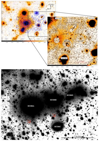
Figure 1. Top panel: An example of ICL in the Fornax cluster in r-band. Left panel: the blue contours are the spatial distribution of the globular clusters derived by [5][6]. Right panel: zoom-in of the west side where it is possible to see how the ICL distributes in the intra-cluster space. Credit: Iodice et al. [1]. Bottom panel: a recent example of ICL (in this case intragroup light) in the HCG 86 group. The grey detection indicated also by red arrows is the detection of the diffuse light. Credit: Ragusa et al. [2].
On the observational side, the most common method used is the “isophotal limit cut-off” (e.g., [7]) in surface brightness, which assumes that the ICL is the remaining component below the cut, after having removed the contribution coming from other sources, such as sky and satellite galaxies. Another method that is increasingly being used lastly relies, instead, on profile fittings with functional forms to model the BCG + ICL component (e.g., [8]).
On the numerical side, given the large amount of information available (not achievable in observations), the ICL can be defined, e.g., by taking advantage of the dynamical information provided by the simulation (e.g., [9]), or by using some binding energy definitions in order to separate all the stars that are not bound to any galaxy (e.g., [10]). Of course, numerical techniques can mimic the observational methods, i.e., surface brightness cut and profile fittings can be reproduced in simulations (see [11][12][13] and many others). Below, I will summarize, by providing some examples, the most common observational and theoretical approaches in separating the BCG from its associated ICL.
1.1. Observational Methods
As mentioned above, the two most common methods to define the ICL observationally rely only on the light that one can observe. The easiest, but not trivial, way to separate the ICL from the rest (after having removed the contribution from other sources, BCG included) is by assuming a cut (different depending on the band) in the surface brightness. Clearly, the cut that can be chosen is quite arbitrary, and there is no value decided a priori that can be adopted as the standard one. This method has been used, and still is, by several authors (see references above). For example, Zibetti et al. [7] analyzed the spatial distribution and color of the ICL by stacking almost 700 galaxy clusters in the redshift range 0.2<z<0.3 taken from the first release of the Sloan Digital Sky Survey. The authors traced the surface brightness profile of the ICL out to 700 kpc and found that it ranges from 27.5 mag/arcsec2 at 100 kpc to down to around 32 mag/arcsec2 at 700 kpc in the r−band. The contribution of the ICL was found to increase with the distance from the center and later studies (e.g., [14][1][15][16] and others) confirmed it.
Despite the common use of this method, it suffers from two non-negligible problems: (1) it does not account for the ICL that overlaps with the BCG in the transition between the two components; (2) the ICL is contaminated by the contribution of large galaxies in the cluster (see, e.g., [17]). Presotto et al. [17] developed a method to obtain refined versions of typical BCG + ICL maps that can be obtained with simple surface brightness cuts. Their method focused mainly on the removal from the map of the light coming from satellite galaxies (the so-called masking). In Figure 2, a comparison is shown between the standard method of surface brightness cut (blue lines and symbols) and the results with their approach (red lines and symbols). They find that the standard surface brightness cut method systematically overpredicts the fraction of ICL as a function of distance from the center, independently of the particular cut used. It must be noted, however, that there are observational studies (e.g., [18] for the Abell 85 cluster) that found the opposite trend, i.e., the surface brightness cut method gives a lower fraction of ICL than, e.g., the profile fitting method. Figure 2 shows also that a standard surface brightness cut has a steep increase from the core to around 100 kpc (in the particular case of MACS J1206.2-0847, which is a massive galaxy cluster at z∼0.4 and part of the CLASH sample [19]) followed by a plateau. On the other hand, Presotto et al.’s masking causes the ICL contribution to drop at large radii, suggesting that most of the ICL is concentrated close to the BCG, which is in good agreement with several recent observational and theoretical results (e.g., [20][21][22][23]).
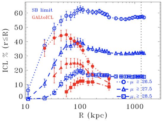
Figure 2. The ICL fraction as a function of distance from the center for different surface brightness cuts and different ICL measurements methods. Blue symbols and lines refer to the standard surface brightness method, while red symbols and lines refer to the method developed in Presotto et al. [17] for masking satellite galaxies. Credit: Presotto et al. [17].
The other most common method consists of using functional forms, such as a double/triple Sersic profile, to fit the light distribution (see references above). There are several ways to achieve it. For example, Montes et al. [18] used the code GALFIT ([24]) to map the 2D distribution of each component, BCG and ICL, with a double Sersic profile (one for each component). Zhang et al. [25] used a triple Sersic profile to 1D fit the azimuthally averaged surface brightness stacked profile of 300 BCG + ICL systems. They found that, as shown in Figure 3, the overall profile can be approximated with the sum of a core, a bulge and a diffuse components (a similar conclusion has been reached earlier by Kravtsov et al. [20]). The three components are dominant at different distances from the center. According to the parameter of the fit by Zhang et al. [25], the core is dominant within 10 kpc, the bulge is dominant between 30 and 100 kpc, and the diffuse component is dominant outside 200 kpc. An advantage of this method lies in the fact that it can separate the two components in a more reliable way than a surface brightness cut where BCG and ICL overlaps, but it is strongly dependent on the functional forms chosen. For instance, Zibetti et al. [7] showed that the distribution of the ICL can be described with an NFW profile [26]. The idea to link the ICL distribution with that of the DM has been used also in theoretical studies such as [27][22][23]. In Contini; Gu [23], the BCG + ICL mass distribution is described by the sum of three different profiles: a Jaffe [28] profile for the bulge, an exponential disk and a modified version of an NFW profile for the ICL.
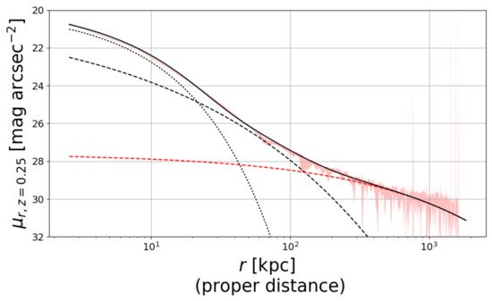
Figure 3. The BCG + ICL light profile from Zhang et al. [25] resulted from the stacking of around 300 clusters at redshift 0.2<z<0.3. The authors found that it can be approximated with three Sersic components (black solid line): a core (dotted line), a bulge (dashed line) and diffuse (red dashed line) components. See text for further details. Credit: Zhang et al. [25].
It is worth mentioning another approach for detecting the ICL that has recently been having some success, a method that makes use of multiscale, wavelet-based algorithms. There are several examples of this approach that have been used in recent years (e.g., [29][30][31][32][33]). One of the latest, just to quote an example, is the code called DAWIS ([33] and references therein). DAWIS is an algorithm, based on wavelet representation, built to restore the unmasked light distribution of given sources as much as possible. Ellien et al. [33] compared the performance of DAWIS with the more common methods described above and found that it can separate the ICL from other sources more efficiently (in the sense that DAWIS performs better) than other methods and is also able to recover a larger quantity of ICL given the way it treats the sky background noise. For readers interested in the details of DAWIS and similar former algorithms of the same family, I refer them to Ellien et al. [33] and references therein.
1.2. Theoretical Methods
Given the fact that, by definition, the ICL component is made of stars that are not gravitationally bound to any galaxy in the cluster, but only to the cluster potential, the natural way to define it would be to find some binding condition such that, all the stars obeying to it can be classified as ICL stars. This condition can be given by the binding energy of star particles with respect to the cluster galaxies. Without entering the details of the method, it is possible to calculate the gravitational potential energy as a function of radius of any given galaxy. In this way, one is able to measure the binding energy of each star particle to each galaxy and collect all those stars that are not bound to any galaxy (see e.g., [11][9][10][34][35]). The collection of these stars will constitute the ICL component of the cluster.
However, despite the binding energy method being efficient in finding stars not bound to satellite galaxies, it does not succeed in separating the BCG from the ICL. Indeed, given the fact that the BCG is placed at the center of the cluster potential, it is not possible to distinguish its mass density profile from that of the cluster itself. In order to completely separate the two components, a few accompanying solutions have been suggested. The most common one has been introduced for the first time by Dolag et al. [9], who used the kinematics of the two components to separate the BCG from the ICL. They found that it is possible to fit the velocity distribution of BCG + ICL with two Maxwellians having different velocity dispersions, and suggested that they correspond to the two components. Figure 4 from Dolag et al. [9] shows the result of their fit: The total velocity distribution of BCG + ICL is marked with a black histogram and its double Maxwellian fit with a grey line. The red and the blue histograms show, instead, the velocity distributions of the BCG and ICL stars, and the corresponding red and blue lines are the two separated Maxwelllians.
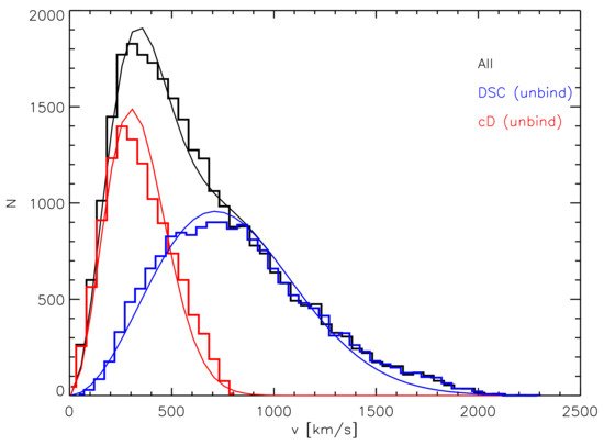
Figure 4. Total velocity distribution of BCG + ICL is marked with a black histogram and its double Maxwellian fit with a grey line. The red and the blue histograms show the velocity distributions of the BCG (called cD in the plot) and ICL (called DSC, diffuse light component, in the plot) stars, and the corresponding red and blue lines are the two separated Maxwellian distributions. Credit: Dolag et al. [9].
Another method usually used in numerical simulations (see, [11][36] and others) relies on the three-dimensional mass density. This method consists of calculating the mass density of each star particle within a sphere of radius equal to the distance of a given N-th nearest neighbor. The further assumption is a threshold density below which the particles can be assigned to the ICL component. The weaknesses of this method lie mainly in identifying ICL particles in high-density regions, and especially in the cluster center. A way to partly overcome this problem has been proposed by Rudick et al. [11], where they look at the density history of each particle, rather than that at a given time, and a particle already classified as ICL remain classified as ICL regardless of its future evolution. Clearly, with respect to the aforementioned method, a density-based approach introduces more free parameters, depending on the level of accuracy that one wants to achieve.
In the list of numerical methods, it is also worth mentioning some semi-analytical approaches. In semi-analytic models, the definition of the ICL does not constitute an issue, given the fact that the amount of ICL is provided by the solution of a set of equations, and its properties depend only on the particular implementation used to describe its formation and evolution. There have been several attempts to describe the formation of the ICL in semi-analytic models, but for the sake of simplicity, I will report only two amongst the most recent.
Guo et al. [37] assumed that the ICL forms from the stellar component of satellite galaxies that are subject to tidal forces after their parent substructures have been totally stripped. These kinds of galaxies are usually referred to as orphans to indicate that their parent subhalo went under the resolution of the simulation. At the pericenter, the main halo density is compared with the average baryon density of the satellite within its half mass radius. If the former is larger than the latter, the satellite is assumed to be disrupted and its stars are assigned to the ICL component. This approach, however, suffers from important limitations. A complete disruption of satellites is less likely than a partial stripping, i.e., some amount of mass stripped. It is indeed more likely that satellite galaxies are subject to several stripping events rather than being totally disrupted in a single one. Moreover, it has been shown that the stripping of the stellar component starts before the complete stripping of the DM subhalo (see, e.g., [38][39]).
A more realistic representation of the stellar stripping was implemented first in Contini et al. [40], then revisited in Contini et al. [41] [42]. In the so-called tidal radius model, the authors assumed that a satellite can lose stellar mass in a continuous way, with several stripping events. The model, at each time step, calculates the tidal radius Rt of the interaction between the cluster potential and the satellite, at the distance of the satellite from the cluster center. A satellite is modeled as a two-component system, bulge and disk. If the tidal radius Rt is smaller than the radius of the bulge, the satellite is assumed to be destroyed, but if it is larger than the bulge radius and smaller than the radius of the satellite, the mass of the disk in the shell between the two radii is stripped and ends up as the ICL component. This method is not only applied to orphan galaxies but also to satellites that still have a DM subhalo. The extra requirement for these satellites is that the half mass radius of the subhalo is smaller than the half mass radius of the disk, which translates into a substantial amount of DM stripped (in accordance with numerical simulations). To account for the stellar mass that gets unbound during galaxy mergers (see, e.g., [10][43][44][45][46] and others), the model also considers the merger channel. At each merger, minor or major, 20% of the stellar mass of the satellite that is merging with the central galaxy is added to the ICL component.
2. Formation Mechanisms
2.1. Pre-Processing
What are we referring to when we use the term pre-processing? Usually, the term pre-processing refers to any material that ended up somewhere but that has been processed elsewhere. The ICL is a clear example of such material. Indeed, part of it has been pre-processed in galaxy groups and then later accreted in clusters. This is a natural consequence of the hierarchical formation of structures. DM haloes continue accreting smaller objects with time, thus increasing their mass. In a very simplified manner, the process can be thought of as follows: at high redshift, DM haloes tend to be smaller and less massive than present day clusters, but galaxies within them start to interact with each other and eventually merge. This lead to the formation of the first ICL stars in galaxy groups (usually called IGL). However, due to the hierarchical nature of the formation of DM haloes, these high redshift smaller haloes will be later accreted by other larger objects, carrying the ICL already formed. In summary, we refer to pre-processed ICL any ICL formed in the past and later accreted (With the term accretion, I mean that the ICL is added to the entire cluster, and becomes part of the ICL already present.). When galaxies were originally centrals, they probably had some ICL associated with them. By being accreted (i.e., they become satellites), they carry their ICL with them, but due to the tidal interactions with the potential well of the new DM halo, their ICL is stripped and becomes part of the diffuse light already present in the accreting halo.
In terms of DM, pre-processing has been shown to be quite an important process. For example, Han et al. [47] found that almost 50% of members in present day clusters were satellites of other hosts, although the fraction depends on the particular mass accretion history of each cluster. Galaxies sit inside DM haloes, so it is natural to expect that a given fraction of the current ICL was produced in the past and then accreted. Contini et al. [40] showed that pre-processing is particularly important for high mass BCGs that reside in clusters, and it can contribute to 30% of the total amount of ICL for the largest BCGs and slightly less than 10% for the smallest BCGs (which are called BGGs when residing in groups), as shown in the top panel of Figure 5.

Figure 5. Top panel: fraction of ICL that has been accreted as a function of the mass of the BCG for different flavors of the model described by Contini et al. [40]. Bottom panel: fraction of the ICL coming from the merger channel as a function of BCG stellar mass. Credit: Contini et al. [40].
A direct example of an ongoing pre-process mechanism is given by the Virgo cluster. Virgo is a nearby galaxy cluster with a moderate richness, and given its vicinity, its structure has been well studied. Precisely its structure makes Virgo an interesting object to study. Virgo can be divided in two subclusters: One of them is centered around M87, a giant elliptical, and the other is centered around another giant elliptical, M49. There are other smaller subclusters that can be identified, such as those surrounding the other two elliptical galaxies, M59 and M60, and a few clouds of galaxies named M, W and W′. Clearly, Virgo is continuing to assemble today and it is far from being at the final stage of its assembly. This makes it particularly interesting for studies that look at the connection between the dynamical state of clusters and their ICL amount and distribution. Mihos et al. [4] recently showed that the W′ cloud in Virgo is a nice example of pre-processing played by groups of galaxies. Indeed, the ICL already formed in the W′ cloud will soon be accreted in the main body of Virgo, and given the strong tidal fields, it will be stripped and dispersed in the global ICL already present.
2.2. Mergers
Another possible mechanism for forming diffuse light is given by galaxy mergers, due to the relaxation processes that take place during the very moment of a merger. Before going into the detail of this channel, it is worth mentioning a caveat. Mergers are not a well-defined process, in the sense that there is not a clear definition of when a merger starts. Of the possible definitions that can be found, all of them would be affected by the fact that part of the stars that will become unbound can actually be classified as belonging to the stripping channel (see discussion in [41]). However, in the final stage of a merger, a given fraction of the stars belonging to the satellite galaxy merging with the central can become unbound and disperse in the ICL component of the cluster.
The literature has plenty of attempts to theoretically model this channel. In hydrosimulations, it is pretty straightforward since it depends on the physical interactions between particles. What is not clear yet, is exactly how to define the moment of when the merger starts, so that particles coming from this channel can be separated from those stripped during the process. Conversely, in semi-analytic models, the definition of a merger is very neat (but it does not necessarily mean the right one), and a merger is defined as the moment when the dynamical friction time of the merging satellite is zero.
Murante et al. [10] focused on the formation of the ICL by means of hydrosimulations and found that most of it (75%) forms through mergers between either the BCG or other massive galaxies, leaving just a small percentage to the stripping channel. On the other hand, Contini et al. [40] showed that the merger channel contributes to the total ICL with just 15%, as shown in the bottom panel of Figure 5 (cyan line), and the rest given by stellar stripping. In Contini et al. [41], the authors argued that this huge difference can be easily explained by the two different definitions of the merger channel used. Indeed, they found that 70% of the ICL coming from stellar stripping is produced in the innermost 100 kpc, a relatively small region within which a satellite can be considered in the process of merging. If they included this part of ICL to the merger channel, they could reach 75%, the same percentage found by Murante et al. [10]. In Contini et al. [40], the authors assumed that 20% of the mass of the satellite galaxy merging with the central ends up in the ICL component. This fraction comes from controlled simulations performed by Villalobos et al. [38], although in reality the fraction can be significantly different from case to case, possibly depending on the orbital circularity, satellite and BCG/halo mass and other important parameters. Similar implementations have also been used in other semi-analytic models (see, e.g., [48][49]).
From the observational point of view, understanding the relative contribution given by mergers to the ICL (and the same for stellar stripping) is far from being easy, simply because it is not possible to trace the past of the ICL stars. However, there are indirect methods that can provide an idea of how much mergers can contribute, and others by looking at the properties of the ICL. For instance, some studies (e.g., [50][51]) pointed out the discrepancy between the observed and predicted stellar mass function, and argued that a possible way to significantly reconcile the two is by invoking a significant mass loss during galaxy mergers, quantified to be around 50% (other theoretical studies, e.g., Contini et al. [52] [53], have shown that the observed and predicted stellar mass functions can be matched by implementing both stellar stripping and mergers (assuming a much lower percentage than 50%).). However, such a high fraction of mass that ends up in the ICL component rather than the BCG seems to be in contrast with the observed properties of the ICL.
2.3. Stellar Stripping
The last important channel for the formation of the ICL is the stellar stripping from galaxies orbiting around the center of the cluster. Stellar stripping applies to all galaxies within a cluster, but tidal forces are responsible for it becoming stronger in the innermost regions close to the cluster center. The efficiency of the stellar stripping, i.e., how strong the interaction between a central galaxy in a halo and a satellite is, depends mainly on two factors: The environment, meaning the mass of the halo and the distance from the center, and the mass of the satellite. The dependence on the latter comes from dynamical arguments. Indeed, due to the dynamical friction [54] that subhaloes (and so galaxies within them) experience when accreted in larger haloes, they orbit around the potential well of the halo by feeling a drag force, caused by the surrounding mass distribution, which tend to slow them down by losing kinetic energy and momentum. This drag force is directly proportional to that mass of satellites, i.e., the biggest travel faster to the center, where they are more likely to be subject to stripping than less massive satellites (see also [55][56][57][58]).
The other important factor for the efficiency of stellar stripping is the environment in which satellites are, and this means the mass of the host halo and the distance from the center. More massive haloes are less concentrated than less massive ones, i.e., groups are more concentrated than clusters (e.g., [55][59][60]). Therefore, the efficiency of stripping is expected to be higher in groups rather than clusters, at least in the innermost regions. However, the tidal radius, that is, the radius at which tidal forces are stronger than the gravity of the satellite, is inversely proportional to the mass of the halo and directly proportional to the mass of the satellite and its distance from the center [61]. This means that, a satellite with the same mass and at the same distance in a group or cluster will experience a larger stripping if it resides in a cluster.
A clear example of the efficiency of stellar stripping in the innermost regions of groups and clusters is given in Figure 6 (from Contini et al. [41]). The left panel shows the cumulative fraction of mass in ICL that has been produced by stellar stripping as a function of distance from the BCG. The solid black line, which represents the median of the distribution, shows that only 10% of the total ICL coming from stellar stripping is built-up at distances farther than 150 kpc, which means that almost all the ICL produced via this channel actually comes from stripping events that happened in the innermost 150 kpc. The right panel of Figure 6 shows the same information shown in the left panel but for two samples of BCGs: less massive than logM∗[M⊙]<11.2 (purple lines), and more massive than logM∗[M⊙]>11.5 (red lines). The panel clearly shows that for more massive BCGs, most of the ICL coming from stellar stripping tends to be produced at larger distances than for less massive BCGs. This result is explained by the trend discussed above, i.e., less massive BCGs are likely to reside in less massive haloes, and these objects are more centrally concentrated than their more massive counterparts.
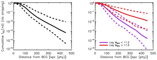
Figure 6. Left panel: cumulative fraction of stellar mass in ICL produced via stellar stripping as a function of distance from the BCG. Right panel: same as left panel, but for BCGs with logM∗[M⊙]<11.2 (purple lines) and BCGs with logM∗[M⊙]>11.5 (red lines). In both panels, solid and dashed lines represent the median, the 16th and 84th percentiles of the distributions, respectively. Credit: Contini et al. [41].
Stellar stripping is stronger in the innermost region of the haloes, and massive satellites (due to dynamical friction) reach that region faster. It is, then, reasonable to expect that they are the most important contributors to the ICL. This prediction was made in Contini et al. [40], and later confirmed by several observations (e.g., [18][14][62][63][64]). In Contini et al. [41], they also looked at what kinds of galaxies contribute the most to the production of ICL via stellar stripping. Figure 7 (from Contini et al. [41]) shows the amount of ICL produced in the innermost 100 kpc via stellar stripping, as a function of the bulge-to-total ratio (left panel), and the amount of mass stripped over the mass of the satellite at the moment of stripping (right panel), for satellite galaxies involved in stripping events. The trend appears pretty clear: disk-like galaxies (B/T < 0.4) contribute the most to the production of ICL, while ellipticals and spheroidals contribute in a marginal way (for details see [41]). The message shown in the right panel is as interesting as the previous one. Indeed, most of the ICL produced by stellar stripping in the innermost 100 kpc comes from small/intermediate stripping events that cut just <30% of the mass of the satellite at the moment of stripping. The total disruption of the satellite is a very unlikely event.
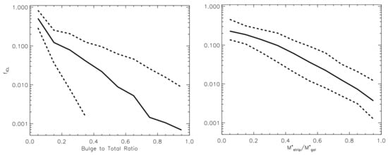
Figure 7. Left panel: fraction of ICL mass via stellar stripping as a function of the bulge-to-total mass ratio of galaxies subject to stripping events, within 100 kpc from the halo center. Right panel: same information as the left panel but as a function of the ratio between the amount of mass stripped and the mass of the satellite at the moment of stripping. In both panels, solid and dashed lines represent the median, the 16th and 84th percentiles of the distributions, respectively. Credit: Contini et al. [41].
All the above theoretical predictions have important consequences on the properties of the ICL. If intermediate/massive satellites, that are likely to be disk-galaxies, contribute the most to the production of ICL via small/intermediate stripping events, it is reasonable to expect that properties of the ICL, such as colors and metallicity, assume given values that are different from those that one would expect if the ICL is mainly produced via mergers or disruption of dwarf galaxies. This is exactly the approach followed by observational studies (e.g., [25][18][14][65][62][64][1]): by looking at the typical colors and metallicity of the ICL, it is qualitatively possible to figure out the process responsible for the formation of the ICL, and the major contributor to it. In addition, by comparing the typical properties of the ICL with those of the BCG, it is possible to learn more about their history. I will address these points in the next section.
References
- Iodice, E.; Spavone, M.; Cantiello, M.; DAbrusco, R.; Capaccioli, M.; Hilker, M.; Mieske, S.; Napolitano, N.; Peletier, R.; Limatola, L.; et al. Intracluster Patches of Baryons in the Core of the Fornax Cluster. Astrophys. J. 2017, 851, 75.
- Ragusa, R.; Spavone, M.; Iodice, E.; Brough, S.; Raj, M.A.; Paolillo, M.; Cantiello, M.; Forbes, D.A.; La Marca, A.; Ago, G.D.; et al. VEGAS: A VST Early-type Galaxy Survey. VI. The diffuse Light in HCG 86 from the Ultra-Deep VEGAS Images. arXiv 2021, arXiv:2105.06970.
- Gu, M.; Conroy, C.; Law, D.; Dokkum, P.V.; Yan, R.; Wake, D.; Bundy, K.; Villaume, A.; Abraham, R.; Merritt, A.; et al. Spectroscopic Constraints on the Buildup of Intracluster Light in the Coma Cluster. Astrophys. J. 2020, 894, 32.
- Mihos, J.C.; Harding, P.; Feldmeier, J.; Rudick, C.; Janowiecki, S.; Morrison, H.; Slater, C.; Watkins, A. The Burrell Schmidt Deep Virgo Survey: Tidal Debris, Galaxy Halos, and Diffuse Intracluster Light in the Virgo Cluster. Astrophys. J. 2017, 834, 16.
- D’Abrusco, R.; Cantiello, M.; Paolillo, M.; Pota, V.; Napolitano, N.R.; Limatola, L.; Spavone, M.; Grado, A.; Iodice, E.; Capaccioli, M. The Extended Spatial Distribution of Globular Clusters in the Core of the Fornax Cluster. Astrophys. J. Lett. 2016, 819, L31.
- Cantiello, M.; D’Abrusco, R.; Spavone, M.; Paolillo, M.; Capaccioli, M.; Limatola, L.; Grado, A.; Iodice, E.; Raimondo, G.; Napolitano, N.; et al. VEGAS-SSS. II. Comparing the Globular Cluster Systems in NGC3115 and NGC1399 Using VEGAS and FDS Survey Data. The Quest for a Common Genetic Heritage of Globular Cluster System. Astron. Astrophys. 2018, 611, A93.
- Zibetti, S.; White, S.; Schneider, D.P.; Brinkmann, J. Intergalactic Stars in z ∼ 0.25 Galaxy Clusters: Systematic Properties from Stacking of Sloan Digital Sky Survey Imaging Data. Mon. Not. R. Astron. Soc. 2005, 358, 949–967.
- Gonzalez, A.; Zabludoff, A.I.; Zaritsky, D. Intracluster Light in Nearby Galaxy Cluster: Relationship to the Halos of Brightest Cluster Galaxies. Astrophys. J. 2005, 618, 195–213.
- Dolag, K.; Murante, G.; Borgani, S. Dynamical Difference Between the cD Galaxy and the Diffuse, Stellar Component in Simulated Galaxy Clusters. Mon. Not. R. Astron. Soc. 2010, 405, 1544–1559.
- Murante, G.; Giovalli, M.; Gerhard, O.; Arnaboldi, M.; Borgani, S.; Dolag, K. The Importance of Mergers for the Origin of Intracluster Stars in Cosmological Simulations of Galaxy Clusters. Mon. Not. R. Astron. Soc. 2007, 377, 2–16.
- Rudick, C.S.; Mihos, J.C.; McBride, C.K. The Quantity of Intracluster Light: Comparing Theoretical and Observational Measurement Techiques Using Simulated Clusters. Astrophys. J. 2011, 732, 48.
- Cui, W.; Murante, G.; Monaco, P.; Borgani, S.; Granato, G.L.; Killedar, M.; Lucia, G.D.; Presotto, V.; Dolag, K. Characterizing Diffused Stellar Light in Simulated Galaxy Clusters. Mon. Not. R. Astron. Soc. 2014, 437, 816–830.
- Tang, L.; Lin, W.; Cui, W.; Kang, X.; Wang, Y.; Contini, E.; Yu, Y. An Investigation of Intracluster Light Evolution Using Cosmological Hydrodynamical Simulations. Astrophys. J. 2018, 859, 85.
- Montes, M.; Trujillo, I. Intracluster Light at the Frontier - II. The Frontier Fields Clusters. Mon. Not. R. Astron. Soc. 2018, 474, 917–932.
- Gonzalez, A.H.; Zaritsky, D.; Zabludoff, A.I. A Census of Baryons in Galaxy Groups and Clusters. Astrophys. J. 2007, 666, 147–155.
- Iodice, E.; Capaccioli, M.; Grado, A.; Limatola, L.; Spavone, M.; Napolitano, N.R.; Paolillo, M.; Peletier, R.F.; Cantiello, M.; Lisker, T.; et al. The Fornax Deep Survey with VST. I. The Extended and Diffuse Stellar Halo of NGC1399 out to 192 kpc. Astrophys. J. 2016, 820, 42.
- Presotto, V.; Girardi, M.; Nonino, M.; Mercurio, A.; Grillo, C.; Rosati, P.; Biviano, A.; Annunziatella, M.; Balestra, I.; Cui, W.; et al. Intracluster Light Properties in the CLASH-VLT Clusters MACS J1206.2-0847. Astron. Astrophys. 2014, 565, A126.
- Montes, M.; Brough, S.; Owers, M.; Santucci, G. The Buildup of the Intracluster Light of A85 as Sees by Subaru’s Hyper Suprime-Cam. Astrophys. J. 2021, 910, 45.
- Postman, M.; Coe, D.; Benitez, N.; Bradley, L.; Broadhurst, T.; Donahue, M.; Ford, H.; Graur, O.; Graves, G.; Jouvel, S.; et al. The Cluster Lensing and Supernova Survey with Hubble: An Overview. Astrophys. J. Suppl. Ser. 2012, 199, 25.
- Kravtsov, A.V.; Vikhlinin, A.A.; Meshcheryakov, A.V. Stellar Mass-Halo Mass Relation and Star Formation Efficiency in High-Mass Halos. Astron. Lett. 2018, 44, 8–34.
- DeMaio, T.; Gonzalez, A.H.; Zabludoff, A.; Zaritsky, D.; Aldering, G.; Brodwin, M.; Connor, T.; Donahue, M.; Hayden, B.; Mulchaey, J.S.; et al. The Growth of Brightest Cluster Galaxies and Intracluster Light Over the Past 10 Billion Years. Mon. Not. R. Astron. Soc. 2020, 491, 3751–3759.
- Contini, E.; Gu, Q. On the Mass Distribution of the Intracluster Light in Galaxy Groups and Clusters. Astrophys. J. 2020, 901, 128.
- Contini, E.; Gu, Q. Brightest Cluster Galaxies and Intracluster Light: Their Mass Distribution in the Innermost Regions of Groups and Clusters. arXiv 2021, arXiv:2014.05913.
- Peng, C.Y.; Ho, L.C.; Impey, C.D.; Rix, H.W. Detailed Structural Decomposition of Galaxy Images. Astrophys. J. 2002, 124, 266–293.
- Zhang, Y.; Yanny, B.; Palmese, A.; Gruen, D.; To, C.; Rykoff, E.S.; Leung, Y.; Collins, C.; Hilton, M.; Abbott, T.M.C.; et al. Dark Energy Survey Year 1 Results: Detection of Intracluster Light at Redshift ∼0.25. Astrophys. J. 2019, 874, 165.
- Navarro, J.F.; Frenk, C.S.; White, S.D.M. A Universal Density Profile from Hierarchical Clustering. Astrophys. J. 1997, 490, 493–508.
- Pillepich, A.; Nelson, D.; Hernquist, L.; Springel, V.; Pakmor, R.; Torrey, P.; Weinberger, R.; Genel, S.; Naiman, J.P.; Marinacci, F.; et al. First Results from the IllustrisTNG Simulations: The Stellar Mass Content of Groups and Clusters of Galaxies. Mon. Not. R. Astron. Soc. 2018, 475, 648–675.
- Jaffe, W. A Simple Model for the Distribution of Light in Spherical Galaxies. Mon. Not. R. Astron. Soc. 1983, 202, 995–999.
- Da Rocha, C.; Ziegler, B.L.; Mendes de Oliveira, C. Intragroup Diffuse Light in Compact Groups of Galaxies-II. HCG 15, 35 and 51. Mon. Not. R. Astron. Soc. 2008, 388, 1433–1443.
- Guennou, L.; Adami, C.; Da Rocha, C.; Durret, F.; Ulmer, M.P.; Allam, S.; Basa, S.; Benoist, C.; Biviano, A.; Clowe, D.; et al. Intracluster Light in Clusters of Galaxies at Redshifts 0.4 < z < 0.8. Astron. Astrophys. 2012, 537, A64.
- Adami, C.; Durret, F.; Guennou, L.; Rocha, C.D. Diffuse Light in the Young Cluster of Galaxies CL J1449+0856 at z = 2.07. Astron. Astrophys. 2013, 551, A20.
- Ellien, A.; Durret, F.; Adami, C.; Martinet, N.; Lobo, C.; Jauzac, M. The Complex Case of MACS J0717.5+3745 and its Extended Filament: Intracluster Light, Galaxy Luminosity Function, and Galaxy orientations. Astron. Astrophys. 2019, 628, A34.
- Ellien, A.; Slezak, E.; Martinet, N.; Durret, F.; Adami, C.; Gavazzi, R.; Rabaça, C.R.; Rocha, C.D.; Pereira, D.E. DAWIS, a Detection Algorithm with Wavelets for Intracluster Light Studies. Astron. Astrophys. 2021, 649, A38.
- Murante, G.; Arnaboldi, M.; Gerhard, O.; Borgani, S.; Cheng, L.M.; Diaferio, A.; Dolag, K.; Moscardini, L.; Tormen, G.; Tornatore, L.; et al. The Diffuse Light in Simulations of Galaxy Clusters. Astrophys. J. 2004, 607, L83–L86.
- Sommer-Larsen, J.; Romeo, A.D.; Portinari, L. Simulating Galaxy Clusters-III. Properties of the Intraclusters Stars. Mon. Not. R. Astron. Soc. 2005, 357, 478–488.
- Rudick, C.S.; Mihos, J.C.; Frey, L.H.; McBride, C.K. Tidal Streams of Intracluster Light. Astrophys. J. 2009, 699, 1518–1529.
- Guo, Q.; White, S.; Boylan-Kolchin, M.; Lucia, G.; Kauffmann, G.; Lemson, G.; Li, C.; Springel, V.; Weinmann, S. From Dwarf Spheroidals to cD Galaxies: Simulating the Galaxy Population in a &ΛCDM Cosmology. Mon. Not. R. Astron. Soc. 2011, 413, 101–131.
- Villalobos, A.; De Lucia, G.; Borgani, S.; Murante, G. Simulating the Evolution of Disc Galaxies in a Group Environment -I. The Influence of the Global Tidal Field. Mon. Not. R. Astron. Soc. 2012, 424, 2401–2428.
- Smith, R.; Choi, H.; Lee, J.; Rhee, J.; Sanchez-Janssen, R.; Sukyoung, K.Y. The Preferential Tidal Stripping of Dark Matter Versus Stars in Galaxies. Astrophys. J. 2016, 833, 109.
- Contini, E.; De Lucia, G.; Villalobos, Á.; Borgani, S. On the Formation and Physical Properties of the Intracluster Light in Hierarchical Galaxy Formation Models. Mon. Not. R. Astron. Soc. 2014, 437, 3787–3802.
- Contini, E.; Yi, S.K.; Kang, X. The Different Growth Pathways of Brightest Cluster Galaxies and Intracluster Light. Mon. Not. R. Astron. Soc. 2018, 479, 932–944.
- Contini, E.; Yi, S.K.; Kang, X. Theoretical Predictions of Colors and Metallicity of the Intracluster Light. Astrophys. J. 2019, 871, 24.
- Conroy, C.; Wechsler, R.H.; Kravtsov, A.V. The Hierarchical Build-Up of Massive Galaxies and the Intracluster Light Since z = 1. Astrophys. J. 2007, 668, 826–838.
- Burke, C.; Collins, C.A.; Stott, J.P.; Hilton, M. Measurements of the Intracluster Light at z ∼ 1. Mon. Not. R. Astron. Soc. 2012, 425, 2058–2068.
- Oliva-Altamirano, P.; Brough, S.; Lidman, C.; Couch, W.J.; Hopkins, A.M.; Colless, M.; Taylor, E.; Robotham, A.S.G.; Gunawardhana, M.L.P.; Ponman, T.; et al. Galaxy And Mass Assembly (GAMA): Testing Galaxy Formation Models Through the Most Massive Galaxies in the Universe. Mon. Not. R. Astron. Soc. 2014, 440, 762–775.
- Zhang, Y.; Miller, C.; McKay, T.; Rooney, P.; Evrard, A.E.; Romer, A.K.; Perfecto, R.; Song, J.; Desai, S.; Mohr, J.; et al. Galaxies in X-Ray Selected Clusters and Groups in Dark Energy Survey Data. I. Stellar Mass Growth of Bright Central Galaxies since z ∼ 1.2. Astrophys. J. 2016, 816, 98.
- Han, S.; Smith, R.; Choi, H.; Cortese, L.; Catinella, B.; Contini, E.; Sukyoung, K.Y. YZiCS: Preprocessing of Dark Halos in the Hydrodynamic Zoom-in Simulation of Clusters. Astrophys. J. 2018, 866, 78.
- Somerville, R.S.; Hopkins, P.E.; Cox, T.J.; Robertson, B.E.; Hernquist, L. A Semi-Analytic Model for the Co-Evolution of Galaxies, Black Holes and Active Galactic Nuclei. Mon. Not. R. Astron. Soc. 2008, 391, 481–506.
- Monaco, P.; Murante, G.; Borgani, S.; Fontanot, F. Diffuse Stellar Component in Galaxy Clusters and the Evolution of the Most Massive Galaxies at z < 1. Astrophys. J. 2006, 652, L89–L92.
- Burke, C.; Hilton, M.; Collins, C. Coevolution of Brightest Cluster Galaxies and Intracluster Light Using CLASH. Mon. Not. R. Astron. Soc. 2015, 449, 2353–2367.
- Groenewald, D.N.; Skelton, R.E.; Gilbank, D.G.; Loubser, S.I. The Close Pair Fraction of BCGs Since z = 0.5: Major Mergers Dominate Recent BCG Stellar Mass Growth. Mon. Not. R. Astron. Soc. 2017, 467, 4101–4117.
- Contini, E.; Kang, X.; Romeo, A.D.; Xia, Q. Constraints on the Evolution of the Galaxy Stellar Mass Function I: Role of Star Formation, Mergers, and Stellar Stripping. Astrophys. J. 2017, 837, 27.
- Contini, E.; Kang, X.; Romeo, A.D.; Xia, Q.; Yi, S.K. Constraints on the Evolution of the Galaxy Stellar Mass Function. II. The Quenching Timescale of Galaxies and its Implication for Their Star Formation Rates. Astrophys. J. 2017, 849, 156.
- Chandrasekhar, S. Stochastic Problems in Physics and Astronomy. Rev. Mod. Phys. 1943, 15, 1–89.
- Contini, E.; De Lucia, G.; Borgani, S. Statistic of Substructures in Dark Matter Haloes. Mon. Not. R. Astron. Soc. 2012, 420, 2978–2989.
- Roberts, I.D.; Parker, L.C.; Joshi, G.D.; Evans, F.A. Mass-Segregation Trends in SDSS Galaxy Groups. Mon. Not. R. Astron. Soc. 2015, 448, L1–L5.
- Contini, E.; Kang, X. Semi-Analytic Predictions of the Mass Segregation from Groups to Clusters. Mon. Not. R. Astron. Soc. 2015, 453, L53–L57.
- Kim, S.; Contini, E.; Choi, H.; Han, S.; Lee, J.; Oh, S.; Kang, X.; Sukyoung, K.Y. YZiCS: On the Mass Segregation of Galaxies in Clusters. Astrophys. J. 2020, 905, 12.
- Gao, L.; Frenk, C.S.; Boylan-Kolchin, M.; Jenkins, A.; Springel, V.; White, S.D.M. The Statistics of the Subhalo Abundance of Dark Matter Haloes. Mon. Not. R. Astron. Soc. 2008, 410, 2309–2314.
- Prada, F.; Klypin, A.A.; Cuesta, A.J.; Betancort-Rijo, J.E.; Primack, J. Halo Concentration in the Standard &Λ Cold Dark Matter Cosmology. Mon. Not. R. Astron. Soc. 2012, 423, 3018–3030.
- Binney, J.; Tremaine, S. Galactic Dynamics: Second Edition; Princeton University Press: Princeton, NJ, USA, 2008.
- DeMaio, T.; Gonzalez, A.H.; Zabludoff, A.; Zaritsky, D.B. On the Origin of the Intracluster Light in Massive Galaxy Clusters. Mon. Not. R. Astron. Soc. 2015, 448, 1162–1177.
- DeMaio, T.; Gonzalez, A.H.; Zabludoff, A.; Zaritsky, D.; Connor, T.; Donahue, M.; Mulchaey, J.S. Lost but not Forgotten: Intracluster Light in Galaxy Groups and Clusters. Mon. Not. R. Astron. Soc. 2018, 474, 3009–3031.
- Montes, M.; Trujillo, I. Intracluster Light at the Frontier: A2744. Astrophys. J. 2014, 794, 137.
- Morishita, T.; Abramson, L.E.; Treu, T.; Schmidt, K.B.; Vulcani, B.; Wang, X. Characterizing Intracluster Light in the Hubble Frontier Fields. Astrophys. J. 2017, 846, 139.