Using the Roeser-Huber formalism, we establish a non-trivial relation between the crystal structure and the transition temperature, Tc, to the superconducting state. By means of this relation, we can calculate Tc for practically all superconducting elements quite accurately within a small error margin. It is shown that this works well also for polymorphic elements and elements under pressure. Furthermore, the Roeser-Huber formalism implies that all calculated data fall on a common line with the slope m1 = h2/(2πkB) = 5.061 × 10−45 m2 kg K, when plotting log(Σ((2x)-2n1-1ML-1))-1 versus 1/Tc, which can be employed as a test when predicting Tc of unknown superconductors.
- Superconducting transition temperature
- elements
- Roeser-Huber formalism
- crystallographic structure
- superconductivity
Topic review
Calculation of the transition temperature of superconducting elements
Subjects: Solid state physics, condensed matter physics, superconductivity
Submitted by:
 Michael Koblischka and Anjela Koblischka-Veneva
Definition
Using the Roeser-Huber formalism, we establish a non-trivial relation between the crystal structure and the transition temperature, Tc, to the superconducting state. By means of this relation, we can calculate Tc for practically all superconducting elements quite accurately within a small error margin. It is shown that this works well also for polymorphic elements and elements under pressure. Furthermore, the Roeser-Huber formalism implies that all calculated data fall on a common line with the slope m1 = h2/(2πkB) = 5.061 × 10−45 m2 kg K, when plotting log(Σ((2x)-2n1-1ML-1))-1 versus 1/Tc, which can be employed as a test when predicting Tc of unknown superconductors.
1. Introduction
Up to now, there are 53 superconducting elements known (in ambient conditions and under pressure, [1,2], and three more are superconductors under special conditions (i.e., in thin film form (Cr), after irradiation (Pd), or C in several modifications [3], e.g., diamond films, alkali-doped fullerene, and carbon nanotubes). A periodic table of the elements with the transition temperature (Tc) data from the literature is presented in Figure 1. From all reviews and teaching books covering this field [2—9], it is clear that there is no simple relation between Tc and the respective crystal structure. Moreover, some elements are polymorphic superconductors with different crystal structures, e.g., La, Hg and Ga, and some elements show changes of the crystal structure under pressure (e.g., Fe becomes superconducting under pressure in the non-magnetic phase (hexgonally close-packed (hcp) ε-Fe phase) [10—12]. Commonly, bandstructure calculations are performed to obtain Tc requiring many parameters (see, e.g., Refs. [13,14] and using given crystal structures as a base, which is, however, not straightforward to enable comparison of a large variety of elements and different crystal structures.
All this demonstrates clearly that the link between the crystal structure and Tc, if existing, must be a much more subtle and non-trivial~one. Exactly this task is fulfilled by the Roeser--Huber (from now on, we use the abbreviation RH) formalism, establishing a truely non-trivial relation between Tc and the given crystal structures.
For a successful application of the RH formalism, one needs the crystallographic information of the possible crystal structures, and about the electronic configuration to count the number NL of electrons involved in superconductivity (the rules for this are similar to the valence electron count used by Matthias [15] and the number of passed (or near) atoms in the crystal unit cell, Natoms as determined from the given crystal structure using the relation l/x < 0.5, which is described in Sec. 2 below.
Thus, a relatively simple calculation procedure like the RH formalism, which requires only knowledge of the crystal structure and the basic electronic configuration with no free parameters, has clear advantages when being incorporated as a test in machine learning approaches to find new superconducting materials [16—18].
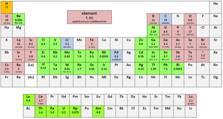
Figure 1. Superconducting elements in the periodic table (light green = superconductor in ambient conditions, light brown = superconductor under applied pressure, and light blue = superconductor with special conditions). Given are the abbreviations of the names, the transition temperatures, Tc, and the applied pressure or some extra info for each element. Hydrogen H is marked in orange concerning the prediction to be a room-temperature superconductor under high pressure. All data given are taken from [1—9]
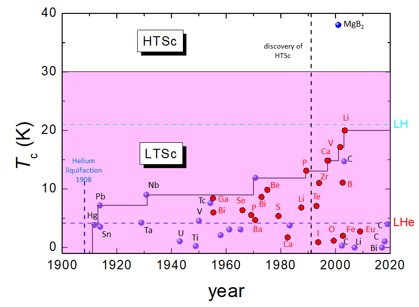
Figure 2. (a) Tc as a function of the year of discovery of the superconducting elements (● – ambient conditions, ● – under pressure). Note the highest Tc of all elements at 20 K for Li under pressure. The borderlines for liquid He (LHe) and liquid H (LH) are also presented. The 30 K-line marks the border between LTSc and HTSc materials, crossed by the alloy superconductor MgB2, which is given for comparison. (b) Logarithmic plot of Tc of various elements in ambient conditions with respect to their crystal structure (body-centered cubic (bcc), face-centered cubic (fcc), hexagonally close-packed (hcp), tetragonal (tetra), monoclinic (mono), orthorhombic (ortho), fcc* and double hexagonally close-packed (dhcp)). The highest Tc in ambient conditions is obtained for Nb with bcc structure, the lowest Tc to date has Bi with a monoclinic structure.
2. Details of the RH formalism
The starting point is the view of a superconducting transition as an integrated resonance curve between the charge carrier wave (Cooper pairs with the deBroglie wavelength λcc) and a characteristic length within the crystal unit cell.
As described already in Refs. [19,20], the Roeser--Huber formula is given as
\begin{equation} \Delta_{(0){\rm ges}}= \frac{h^2}{2 M_{\rm L}} \cdot \left(\sum_{R_1}^{R_n} \frac{1}{(2 x_{R_i})^2} \cdot n_0^{2/3} \cdot \frac{n_{2R_i}}{n_{1R_i}}\right) = \pi k_B T_{c(0)} ~~~, \label{eq:1} \end{equation} with Δ(0) describing the lowest level energy of the PiB. h denotes the Planck constant, kB the Boltzmann constant, ML is a parameter with the unit of a mass, and the sum is taken for all possible directions, Ri, as explained below. For all unit cells of metallic elemental superconductors, there are no 2D-like superconducting planes, thus n0 (describing the number of superconducting planes of 2D superconductors) is set to n0 = 1, and the parameter n2 is also set to 1 as the simple crystal structures of the elements do not have multiple superconducting paths as in the case of alloys [20,21].
The characteristic interatomic distance x now depends on each crystallographic direction (which will be called superconducting path hereafter), Ri, and the correction factor, n1, the determination of which is discussed below.
It is to the credit of the late Prof. Roeser and his students to have established a set of rules which provide the essential input for the calculations.
Following the works of Moritz [19] and [21] Stepper, there are four important points to be considered when calculating Tc for metallic elements:
# The distance x corresponds to an interatomic distance similar to the particle-in-box (PiB) approach applied in [22,23]. The distance x is obtained from possible symmetric paths (also called superconducting directions in the following) for the movement of the charge carrier wave within the crystal structure, as discussed below. The crystallographic data come from respective databases [24,25], which is an important issue for application of the RH formalism in machine-learning calculation approaches.
# The parameter ML for high-Tc superconductor (HTSc) compounds was taken as 2 me (= electron mass, 2 for a Cooper pair). For element superconductors, ML= η me is much higher as all the phononic interactions (Fermi temperature, Debye temperature, effective mass, charge carrier density) are incorporated in the parameter η. In a first approximation, η me ~1900, which corresponds closely to the mass of a proton (mp/me = 1836.15). Regarding the location of metallic superconductors in a Uemura plot (Tc as function of the Fermi temperature, TF = (m* vF2)/(2 kB) [26,27] and vF denoting the Fermi velocity, m* is the effective mass) in the lower right corner with TF ~104.105 K, the high value for η is reasonable. This significant difference between elemental metallic superconductors and the HTSc materials was also pointed out by Emery and Kievelson [28] mentioning the substantial phase rigidity of the superconducting state in, e.g., lead at all temperatures below Tc.
# A first correction factor is required to account for more complex crystal structures. Atoms being close to a superconducting direction may have an influence on the moving charge carriers via the phonon interaction. Therefore, the number of atoms passed within a unit cell is counted. This correction was originally added to the parameter ML via:
\begin{equation} M_L = \frac{N_L}{N_{\rm atoms}} \cdot m_p ~~~, \label{eq:2} \end{equation}
which we keep here for consistency. Regarding the definition of η given above, the relation NL/Natoms is thus incorporated in η.
Here, NL represents the number of the charge carriers and Natoms denotes the number of the near, passed atoms along each superconducting path. A correction factor n1 can be then defined as n1 = NL/Natoms. In case there are no (near) passed atoms, then n1 = 1.
As the symmetry of the superconducting path plays an important role for our considerations, the passed atoms must be symmetrically arranged along the superconducting path, as otherwise the charge carriers would be not in phase due to the unsymmetric forces. This implies that superconductivity cannot exist in directions with unsymmetrically arranged passed atoms. As test for the influence of the passed atoms, we define a relation l/x, with l being a distance perpendicular to the direction of the moving charge carriers. If l/x ≤ 0.5, the passed atoms show an influence on the superconductivity and must be counted in Natoms.
Here, it is important to point out that NL and Natoms are not free parameters, but are given from the respective crystal structure being investigated. A special case for determining NL will be encountered for hcp Fe under pressure as discussed below.
# A second correction factor is necessary to account for anisotropic superconductivity, which can even lead to so-called multimode superconductivity. The factor n2 gives a relation between the specific directions for the charge carrier wave, Ri, in the given crystal structure.
The energy Δ(0) and the transition temperature Tc(0) are then calculated for each existing superconducting path Ri, and the results must be summed up according to Equation (1). If one of the directions Ri gives a reasonable value for Tc(Ri) to compare with the experimentally determined Tc, this direction is taken as the superconducting path. However, the Tc(Ri)-values of the other directions and the complete sum of all Tc(Ri) may also have important implications as, e.g., in the case of Al, which was discussed in Ref. [20], the experimental value of Tc is reached with 2 of the possible 4 directions in the fcc structure, but the total sum of all 4 directions is strikingly close to the increased Tc, when measuring thin films. A similar situation is given for the energies, Δ(0)(Ri). Δ(0)(Ri) may be compared to the pairing energy or energy gap as determined experimentally.
Thus, all Δ(0)(Ri)- and Tc(Ri)-values must be calculated for a given material.
For most elemental superconductors, n2 = 1, in contrast to the metallic alloys Nb3Sn or MgB2, where superconducting directions can exist several times within one unit cell, as already discussed in Ref. [20].
The Roeser--Huber formalism (1) does not contain any free parameters, as all the required inputs are given via the crystal unit cell (i.e., x and Natoms) and NL from the basic electronic configuration of the material. It must be noted here that the RH formalism does not describe how the Cooper pairs are formed, and so it is not possible to determine if a given material is a superconductor. However, regarding the limits of the parameter η (ηmin = 2, and ηmax is set by the demand of the BCS-theory that the effective charge carrier mass, m* cannot be smaller than m*< 0.1 me for isotropic, spherical Fermi surfaces [29], one may deduce a possibility to judge if superconductivity for a given material and crystal structure exists. This will be elaborated in future works.
Figure 3 presents the Roeser--Huber plot with many calculated superconducting materials, high-Tc superconductors (HTSc, marked with a red circle), metallic alloys (blue circle) and elements (green circle). Practically all superconducting elements can be calculated using the RH formalism with only small error margins. The only exceptions are the very low-Tc materials Li, Be and Bi, where the low values of Tc can only be reproduced with an adaptation of η, which is due to either an extremely small charge carrier mass (Li, Be) or a large electron mean free path (Bi). In contrast, the RH formalism works well to calculate the respective Tc-values of the same materials under applied pressure.
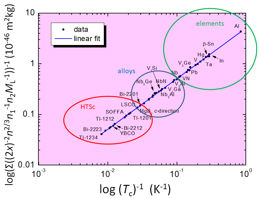
Figure 3. The Roeser--Huber plot for a large number of superconducting materials. Red circle: HTSc, blue circle: alloys, and green circle: elemental superconductors. Some overlaps between these regions do exist. For clarity, only some of our collected data are included.
A very important point is here that all the data of Tc obtained fall on a common, straight line (blue), which follows the equation for a particle in a box [23] with the slope h2/(2π kB) = 5.061 × 10-45 m2 kg K. This result enables the RH formalism to act as a test for given predictions of Tc, e.g., for the case of metallic hydrogen as was done recently in Ref. [30].
3. Conclusions
To conclude, in our article [31] and before in Ref. [20], we have presented calculations of the superconducting transition temperature, Tc, for two polymorphic superconducting elements (Hg, La) using the RH formalism and for ε-Fe (hcp) under pressure. The principles of this formalism enable to reproduce the different Tc-values of various crystal structures of the same elements, which directly proofs the validity of the concept. This will enable us to apply this formalism for the prediction of Tc of still unknown superconducting materials, e.g., in machine learning approaches.
This entry is adapted from 10.3390/met12020337
References
- Flores-Livas, J.A.; Boeri, L.; Sanna, A.; Profeta, G.; Arita, R.; Eremets, M. A perspective on conventional high-temperature superconductors at high pressure: Methods and materials. Phys. Rep. 2020, 856, 1—78.
- Buzea, C.; Robbie K. Assembling the puzzle of superconducting elements: A review. Supercond. Sci. Technol. 2005, 18, R1—R8.
- Buckel, W., Kleiner, R. Supraleitung. Grundlagen und Anwendungen, 7th edition, Wiley-VCH, Weinheim, 2013.
- Eisenstein, J. Superconducting elements. Rev. Mod. Phys. 1954, 26, 277—291.
- Matthias, B. T. Chapter V: Superconductivity in the Periodic System. Prog. Low Temp. Phys. 1957, 2, 138—150.
- Roberts, B. W. Survey of superconductive materials and critical evaluation of selected properties. J. Phys. Chem. Ref. Data 1976, 5, 581—821.
- Poole, C.P. (Ed.) Handbook of Superconductivity, 1st ed.; Elsever: Amsterdam, The Netherlands, 1995.
- Narlikar, A. V. Superconductors. Oxford University Press, Oxford, U.K., 2014.
- Savitskii, E.M.; Baron, V.V.; Efimov, Y.V.; Bychkova, M.I.; Myzenkova, L.F. Superconducting Materials, 1st ed.; Plenum Press: New York, NY, USA; London, UK, 1973.
- Shimizu, K.; Kimura, T.; Furomoto, S.; Takeda, K.; Kontani, K.; Onuki, Y.; Amaya, K. Superconductivity in the non-magnetic state of iron under pressure. Nature 2001, 427, 316—318.
- Steinle-Neumann, G.; Stixrude, L.; Cohen, R. E. Magnetism in dense hexagonal iron. Proc. Natl. Acad. Sci. 2004, 101, 33—36.
- Roth, S. Theoretical Investigation of One-Component-Superconductors and their Relationship between Transition Temperature and Ionization Energy, Crystal Parameters and Further Parameters. Ph.D. Thesis, Institute of Space Systems, University of Stuttgart, 2018. (in German)
- Nowotny, H.; Hittmair, O. Calculation of the transition temperature Tc of superconductors. Phys. Stat. Solidi (B) 1979, 91, 647—656.
- Arita, R.; Koretsune, T.; Sakai, S.; Akashi, R.; Nomura, Y.; Sano, W. Nonempirical Calculation of Superconducting Transition Temperatures in Light-Element Superconductors. Adv. Mater. 2017, 29, 1602421.
- Matthias, B. T., Geballe, T. H., Compton, V. B. Superconductivity. Rev. Mod. Phys. 1963, 35, 1—22.
- Stanev, V., Oses, C., Kusne, A. G., Rodriguez, E., Paglione, J., Curtarolo, S., Takeuchi, I. Machine learning modeling of superconducting critical temperature. npj Computational Materials 2018, 4, 29.
- Lee, D.; You, D.; Lee, D.; Li, X.; Kim, S. Machine-Learning-Guided Prediction Models of Critical Temperature of Cuprates. J. Phys. Chem. Lett. 2021, 12, 6211—6217.
- Konno, T.; Kurokawa, H.; Nabeshima, F.; Sakishita, Y.; Ogawa, R.; Hosako, I.; Maeda, A. Deep learning model for finding new superconductors. Phys. Rev. B 2021, 103, 014509.
- Moritz, A. Calculation of the transition temperature of one-component-superconductors. Master thesis IRS 09-S33, Institute of Space Systems, University of Stuttgart, Stuttgart, Germany, 2009. (in German)
- Koblischka, M. R., Roth, S., Koblischka-Veneva, A., Karwoth, T., Wiederhold, A., Zeng, X. L., Fasoulas, S., and Murakami, M. Relation between Crystal Structure and Transition Temperature of Superconducting Metals and Alloys. Metals 2020, 10, 158.
- Stepper, M. Master thesis IRS 08-S23, Institute of Space Systems, University of Stuttgart, Germany, 2008. (in German)
- Roeser, H. P., Hetfleisch, F.; Huber, F. M., Stepper, M., von Schoenermark, M. F., Moritz, A., Nikoghosyan, A. S. A link between critical transition temperature and the structure of superconducting YBa2Cu3O7-δ. Acta Astronautica 2008, 62, 733—736.
- Rohlf, J. W.: Modern Physics from α to Z0. Wiley, New York (1994).
- ICDD. ICDD PDF Data Base; ICDD: 12 Campus Blvd, Newtown Square, PA 19073, USA (accessed on 12. 02. 2022).
- Materials Project Database V2019.05. Available online: https://materialsproject.org/ (accessed on 12. 02. 2022).
- Uemura, Y. J.; Le, L. P.; Luke, G. M.; Sternlieb, B. J.; Wu, W. D.; Brewer, J. H.; Riseman, T. M.; Seaman, C. L.; Maple, M. B.; Ishikawa, M.; Hinks, D. G.; Jorgensen, J. D.; Saito, G.; Yamochi, H. Basic Similarities among Cuprate, Bismuthate, Organic, Chevrel-Phase, and Heavy-Fermion Superconductors Shown by Penetration Depth Measurements. Phys. Rev. Lett. 1991, 66, 2665—2668.
- Uemura, Y. J. Condensation, excitation, pairing, and superfluid density in high-Tc superconductors: the magnetic resonance mode as a roton analogue and a possible spin-mediated pairing. J. Phys.: Condens. Matter 2004, 16, S4515—S4540.
- Emery, V. J.; Kivelson, S. A. Importance of phase fluctuations in superconductors with small superfluid density. Nature 1995, 374, 434—437.
- Talantsev, E. F.; Mataira, R. C.; Crump, W. P. Classifying superconductivity in Moiré graphene superlattices. Sci. Rep. 2020, 10, 212.
- Ghosh, K. J. B.; Kais, S.; Herschbach, D. R. Dimensional interpolation for metallic hydrogen. Phys. Chem. Chem. Phys. 2021, 23, 7841—7848.
- Koblischka, M. R.; Koblischka-Veneva, A. Calculation of Tc of superconducting elements with the Roeser-Huber formalism. Metals