The Physics of Flows in a Curved Channel

The Physics of Flows in a Curved Channel: Comparison

Please note this is a comparison between Version 1 by Yeganeh Saffar and Version 2 by Jason Zhu.

Microchannels with curved geometries have been employed for many applications in microfluidic devices in the past decades. The Dean vortices generated in such geometries have been manipulated using different methods to enhance the performance of devices in applications such as mixing, droplet sorting, and particle/cell separation. Understanding the effect of the manipulation method on the Dean vortices in different geometries can provide crucial information to be employed in designing high-efficiency microfluidic devices.

Dean flow
curved microchannel
particle sorting

1. Introduction

The velocity profile and flow structure of the Poiseuille flow in a channel with a circular cross-section and an initial radius of curvature

R_{c} = \infty

(straight channel) is shown in Figure 1a ^[1][2][55,56]. In the straight section, the velocity profile is axisymmetric and the maximum velocity point is on the centerline of the channel ^[3][4][57,58]. Circular constant velocity contours in a channel with a circular cross-section are concentric with the channel cross-section, as shown in Figure 1c ^[3][4][57,58]. The symmetrical shape of the channel walls and cross-section balances the velocity and pressure gradients and generates a symmetrical flow diagram ^[3][4][57,58].

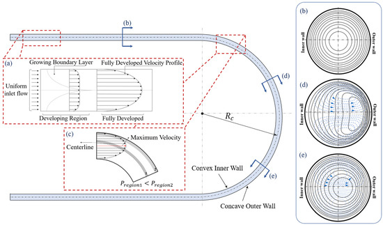
Figure 1. Flow in a curved channel: (a) velocity profile of the developing and developed flow in a straight channel far from the curved section, (b) constant velocity lines of the flow in the straight section of the channel, (c) unsymmetrical velocity profile of the Dean flow entering the curved section of the channel, (d) constant velocity lines of the flow in the entrance of the curved section, (e) further into the curved section where the center of the vortices are shifted more toward the concave wall.

Berger et al. ^[5][59] highlighted that investigations into the physics of the flow inside curved channels began in the early 1900s. In 1902, an experimental observation in a curved pipe determined that the location of the maximum velocity moves toward the concave outer wall ^[6][60]. Later, Eustice (1910, 1911) injected ink into water passing through a pipe and used its streamline motion to demonstrate the existence of the secondary flow ^[7][8][61,62]. In 1928, for the first time, Dean ^[9][10][47,63] realized that in a pressure-driven system, the flow rate slightly decreases when increasing the channel curvature’s radius. For low velocity flows in a curved channel with the Reynolds number

R e = ρ U d / μ < 2000,

where $ρ$ is fluid density, $U$ is the uniform velocity, $d$ is the hydraulic diameter of the channel, and $μ$ is the dynamic viscosity, it was proposed that the radius of curvature is proportional to variations in the flow rate through the parameter, $K$ , defined as:

(1)

In this equation,

d

is the hydraulic diameter of the channel and

R_{c}

is the average of the radius of the curvature of the walls ^[9][47].

A fully developed flow entering a curved channel develops a centrifugal force in an asymmetrical geometry ^[11][64]. Such asymmetricity affects the parabolic velocity profile and causes a shift in the location of the maximum velocity compared to a straight microchannel ^[12][65]. Therefore, the maximum velocity shifts from the centerline toward the concave outer wall and forms an asymmetric velocity profile ^[5][13][59,66], as depicted in Figure 1c. This velocity profile induces a high pressure difference between the location of maximum velocity and the concave wall as

P_{r e g i o n 2} > P_{r e g i o n 1}

^[2][14][56,67]. This induced pressure gradient results in a transverse flow motion on the channel centerline. As a result of this transverse motion, a secondary flow is formed in the flow field ^[2][12][14][56,65,67]. The secondary flow causes an energy loss from the main flow stream in the curved channel, which increases the required pressure difference for a certain flow rate compared to a straight channel with the same cross-sectional area. As a result, with a constant pressure difference between the inlet and outlet of a channel, the flow rate in the curved channel will be less than that of the straight channel ^{[2][9][12][14]}[47,56,65,67].

In sections (d) and (e) of the curved channel of Figure 1, flow streamlines and constant velocity contours in the cross-section of a curved channel are shown ^[15][16][68,69]. With an increase in the velocity, the constant velocity contour lines, shown by the solid lines in Figure 1b, start to deform from circles into bended ovals leaning towards the concave outer wall. The flow streamlines show that the secondary flow pattern forms as two symmetrical and counter-rotating vortices on the top and bottom of the channel ^[5][16][59,69]. These vortices are known as the primary Dean vortices ^[5][16][59,69]. It is shown that, for a higher velocity, the pressure gradient between the slow-pressure zone close to the concave outer wall and the high-pressure zone close to the convex inner wall is higher ^[5][9][16][47,59,69]. Consequently, as the velocity increases the center of the vortices shifts towards the concave outer wall ^[16][69].

In terms of the scale, the principles of the Dean flow remain the same for micro- and macroscales. However, the specific details and considerations may differ. At the micro-scale, such as in microfluidics, the channels typically have dimensions in the order of tens to hundreds of micrometers ^[17][18][70,71]. At such a scale, the flow characteristics in the microchannel may exhibit unique behaviors due to the dominance of viscous forces over inertial forces ^[19][20][49,72]. Consequently, the Reynolds number (the ratio of inertial forces to viscous forces) may be much lower in microchannels ^[12][65]. At the macroscale, such as in larger channels or pipes, the Dean flow is still present. However, the relative importance of inertial forces increases compared to the viscous forces. Thus, the Reynolds number is typically higher at the macroscale, and inertial effects play a more significant role in the dynamics of the flow ^[19][49].

2. The Dean Number

The non-dimensional parameter,

K

in Equation (1) was introduced by Dean ^[9][47] to investigate the effect of channel curvature on flow. This parameter was later named after its founder as the Dean number,

D e

^[5][59]. This dimensionless number indicates the relationship between the channel geometry and the reduction in flow rate in curved channels ^[5][59]. In addition to Dean’s definition in Equation (1), there are several other variations of this equation developed by other researchers.

Theoretical investigations typically deploy either the mean velocity of the channel or pressure gradient as the driving factor to calculate the Dean number. In experimental studies, using the mean velocity is more common since it is more convenient to measure velocity than the pressure gradient, considering the fact that, in complex flow geometries, the pressure gradient changes in different directions. However, for a fully developed flow, the differences between calculations based on the mean axial velocity and pressure gradient are minor ^[5][59]. Therefore, in numerical studies, the pressure gradient is usually used instead of the mean velocity estimation to reduce the uncertainty of the calculations ^[7][61].

The inconsistency in the definition of geometrical parameters such as the measure of the radius of curvature based on the convex wall, concave wall, or centerline of the channel, is another reason for the various definitions of De. Thus, it is always important to identify the equation that each study has used to calculate the

D e

since in a similar case using a different definition can cause disagreement between the results. Comparing the results from different studies without considering the calculation references can lead to incorrect conclusions. As a result, it is necessary to study the definitions of De and their differences based on their applications.

Most of these equations use similar parameters, such as the Reynolds number,

R e

, based on the hydraulic diameter of the channel and its inlet velocity;

R_{c},

the radius of curvature; and

d

, the width of the channel, in their definitions. But they are slightly different, with an additional constant coefficient or a constant power.

3. Dean Number Thresholds

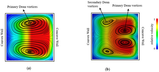
Various dominant or temporary configurations of Dean vortices can be formed by changing the flow or geometric parameters. The appearance of these configurations can be characterized by the Dean number ^[13][21][66,79]. When increasing the Dean number from 0, the first configuration of Dean vortices, a pair of counter-rotating vortices, appears and are called the primary Dean vortices. An example of these is shown in Figure 2a ^[11][12][64,65], in a radial cross-section view of a curved channel with a rectangular cross-section. The first Dean number threshold in which the vortices appear for the first time is termed the initial Dean number,

D e_{i}

Increasing the Dean number such that $D e_{i} < D e$ leads to an increase in the transverse velocity of the flow and the strength of the vortices generated. This can be achieved by increasing the flow rate such that the maximum velocity location moves further toward the concave wall, as is depicted in Figure 2b. As a result, the core of the Dean vortices shifts to the concave wall ^[11][12][64,65]. With further increasing of the Dean number, two secondary Dean vortices detach from the main vortices. These secondary vortices are smaller than the main/primary vortices. Figure 2b shows a flow configuration including primary and secondary Dean vortices. The Dean number at which the secondary Dean vortices start to form is called the critical Dean number, $D e_{c}$ ^[12][22][23][65,80,81].

Figure 2. Visualization of the out of plane velocity contours on the background and Dean vortices shown by streamlines inside a rectangular channel. (a) Formation of the primary Dean vortices. (b) Formation of the secondary Dean vortices.

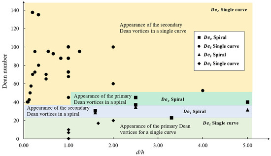
The values of the initial and critical Dean numbers depend on various factors such as the aspect ratio (

d / h

), which is defined as the ratio of the channel width or diameter,

d

, to the height,

h

, and the radius of curvature,

R_{c}

^[12][21][65,79]. Being a function of several parameters makes it difficult to predict the flow configuration in a geometry at a given flow state without numerical or experimental investigations. The values of the Dean numbers, which are all recalculated based on (8), and the channel cross-sectional aspect ratios for different curve and spiral microchannel geometries have been derived from the literature and presented. These values are used to generate the phase map shown in Figure 3., which compares De against the channel aspect ratio, d/h. The color variance in the map differentiates the regions of appearance of different Dean vortices. It can be determined from this figure that in a single curve geometry with various channel widths or radii of curvatures, as shown in Figure 3, the initial Dean number is in the range of

0 < D e_{i} < 20

, while the critical Dean number is in the range of

100 < D e_{c} < 160

. For spiral microchannels, the range is significantly different for the initial and critical De than the single curve channel case. Both the initial and critical Dean numbers for spiral cases are close to each other, in the range of

20 < D e_{i} < 50

Figure 3. Critical and initial Dean numbers in single and multiple curved geometries, demonstrating the effect of the channel shape in addition to other geometrical properties ^{[1][12][22][24][25][26][27][28][29][30][31]}[55,65,77,80,82,83,84,85,86,87,88].

It is shown in Figure 3 that the critical and initial Dean number (using the same Dean number definitions for all data sets) for a spiral geometry are located in a very small range in the low Dean number area, which indicates a small window for the appearance of two primary Dean vortices. The initial Dean number of a single curve is in the same area and about half of the initial Dean number of a spiral. This means that the Dean vortices can be generated at lower velocities in a single curve. The critical Dean number for a single curve is found to be in the high Dean number area and almost three times bigger than the initial Dean number for the same geometry.