Your browser does not fully support modern features. Please upgrade for a smoother experience.
Please note this is a comparison between Version 2 by Catherine Yang and Version 1 by Jiyeong Lee.
Advancements in data-acquisition technology have led to the increasing demand for high-precision road data for autonomous driving. Specifically, road boundaries and linear road markings, like edge and lane markings, provide fundamental guidance for various applications. Unfortunately, their extraction usually requires labor-intensive manual work, and the automatic extraction, which can be applied universally for diverse curved road types, presents a challenge.
- automatic extraction
- OBB collision-detection algorithm
- road boundary
- road marking
1. Creating Oriented Bounding Box of Road Boundaries Using Normal Vector
In many studies, a bounding box specifies spatial locations and classes (e.g., cars and trees). A bounding box is widely used in point cloud data to simplify the complex set of points as a representative box and apply collision detection [41][1]. Among the several types of bounding boxes, the oriented bounding box (OBB) is the smallest rectangle with an inclined axis around the object (Figure 31). In contrast, an axis-aligned bounding box (AABB) is a minimum bounding hexahedron that envelops an object and conforms to a set of fixed orthogonal axes. Owing to its simple geometry, the AABB has less memory and is tested faster (Figure 31). However, describing the directional information of a given object is difficult.

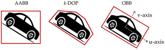
Figure 31. Comparing three types of bounding boxes: axis-aligned bounding box (AABB), k-discrete-orientation polytope (k-DOP), and oriented bounding box (OBB).
Comparing three types of bounding boxes: axis-aligned bounding box (AABB), k-discrete-orientation polytope (k-DOP), and oriented bounding box (OBB).
In contrast, a discrete-orientation polytope (DOP) is a bounding polyhedron defined with the k number of axes. DOP can bind the object better than AABB but requires more memory (Figure 31). Comparing these two bounding boxes, the OBB is the optimal bounding box for road marking extraction regarding memory and direction information.
To generate OBBs, it is essential to establish a set of basis axes and u- and v-axes (Figure 31). The u-axis was aligned in the direction of the OBB, which acted as a reference line for defining the OBB, and the v-axis was perpendicular to the u-axis. For the OBBs of the road boundaries, the u-axis can be extracted by identifying the boundary line of the floor plane consisting of points with a normal vector of 90°. Therefore, the u-axis can be determined with the edge of the plane, which defines the OBB of the road boundaries.
A floor plane can be generated by identifying the lowest points in the search area. Applying the search area can decrease the randomness and noise in the point cloud data. In particular, this search step determined the lowest points because the lowest point of the point clouds collected from the MMS represents the road surface. Therefore, defining the proper size and location of the search area is essential in terms of accuracy and conformity to extract the edge because it ends up being a reference line aligned with the u-axis of the OBB. The radius of the search area was set as 50 cm (Figure 42b). If it is set to a radius of 1 m, the road’s curvature is ignored; instead, a straight line is generated (Figure 42a).
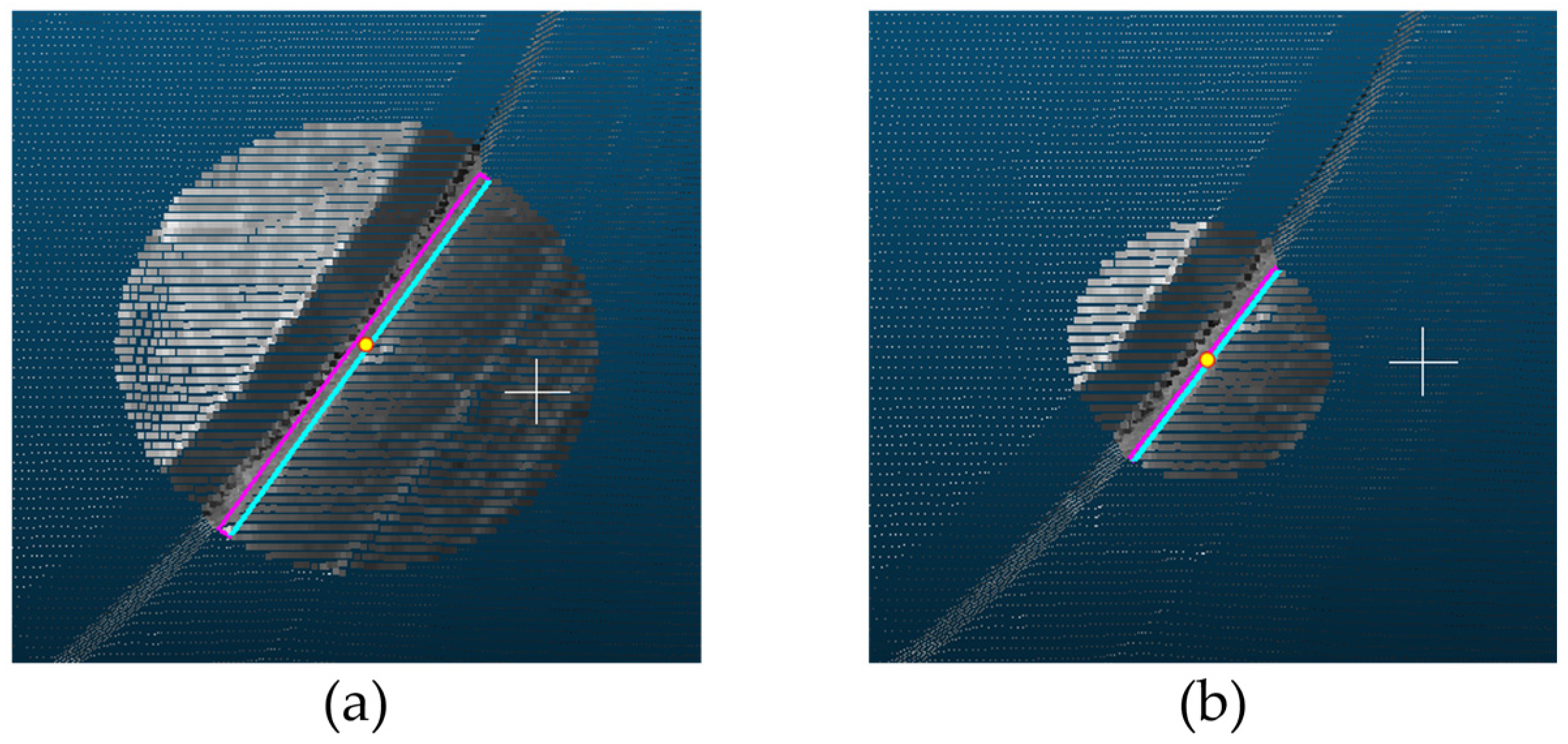

Figure 42.
(
a
) The radius of the search area is 1 m. (
b) The radius of the search area is 50 cm.
) The radius of the search area is 50 cm.
The location of the search area is also associated with not only the accurate extraction of the u-axis reference line of the OBB but also the generation of the road surface. Selecting the proper location of the search area can eliminate the need to pre-process the point cloud data. To generate an accurate reference line for the OBB, the search area should be located where the following conditions should be met: first, the boundaries of the road surface are clear, the direction can be confirmed, and the data should be acquired in areas with no lost data. For example, when the position of the search area is such that the boundary is identified, as shown in Figure 53a, the reference line for creating an OBB can be extracted accurately, as shown in Figure 53b.
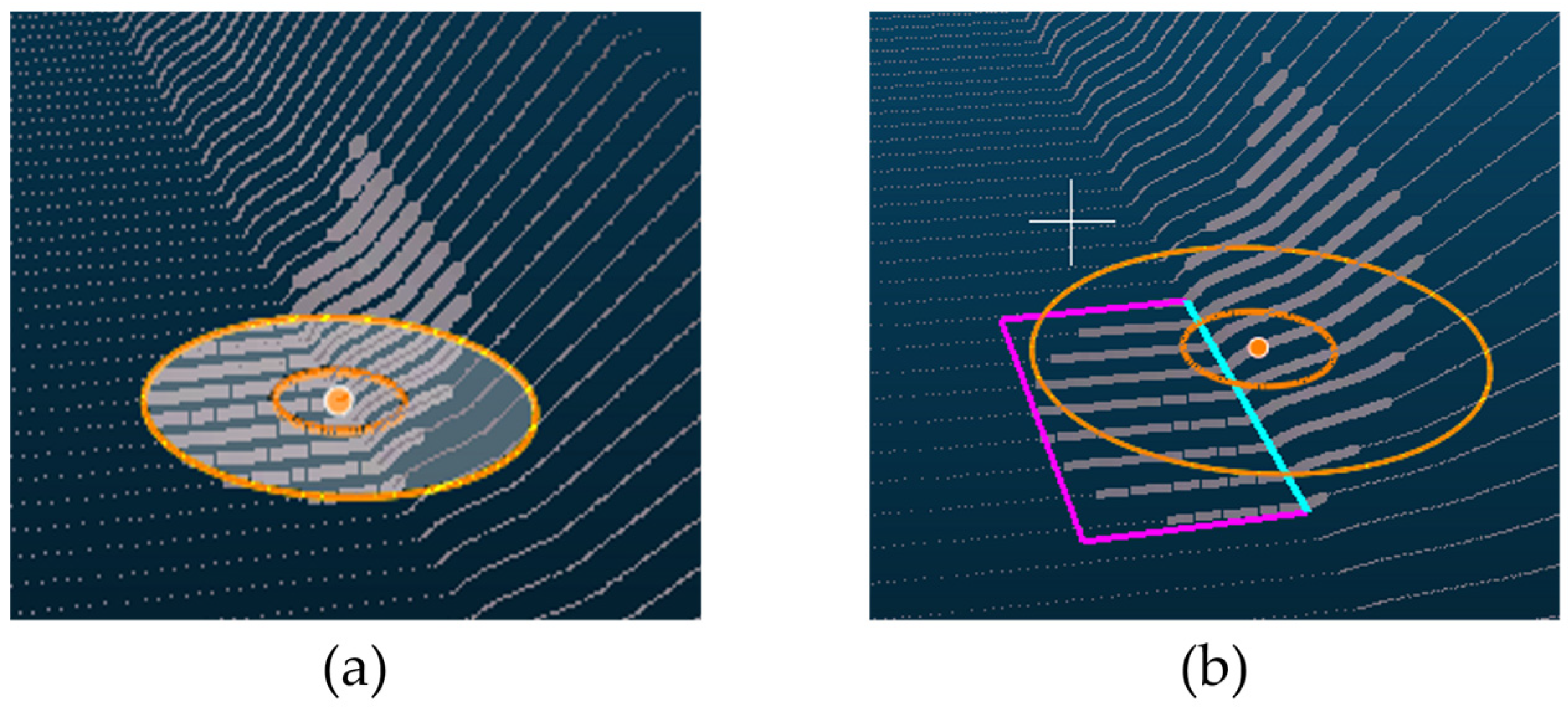
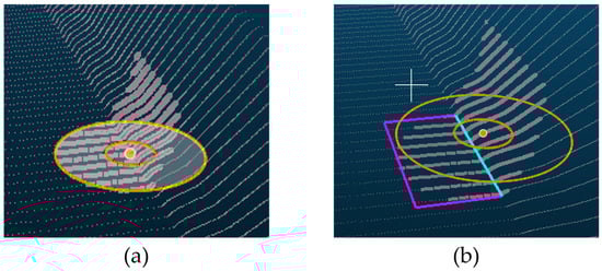
Figure 53.
(
a
) Setting a search area (the large orange circle in (
a
) to extract a bottom plane. (
b
) Detecting the edge of the plane by setting the search area to include both the road surface and the boundary. The extracted edge of the plane (the sky-blue line in (
b
)) is a reference line for the oriented bounding box (OBB) (the pink rectangle in (
b)).
)).
Moreover, it is essential to encompass both road boundary and road surface within the search area. If the search area is located outside an area not in contact with the road boundary, the edge detection causes errors, as shown in Figure 64a. Moreover, if all the portions of the search area occupied the road surface, they failed to identify the edges (Figure 64b).
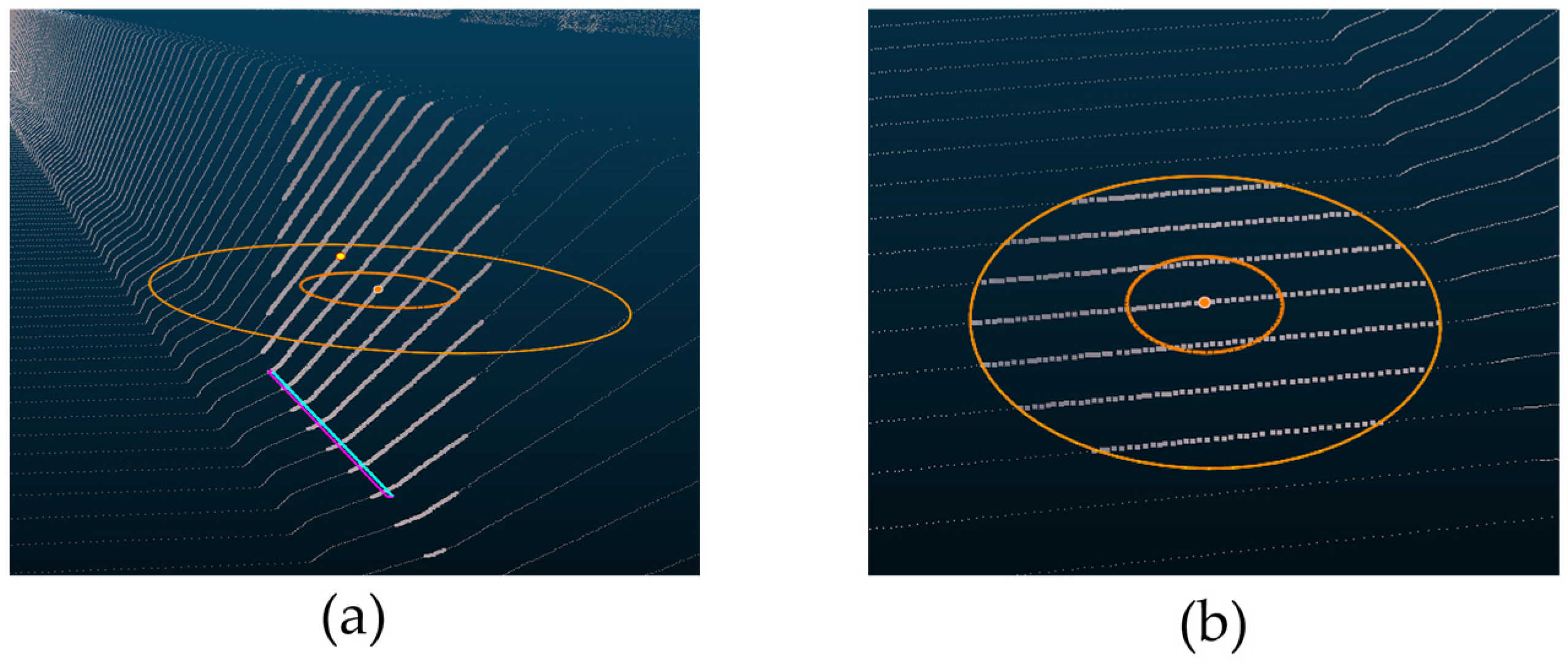
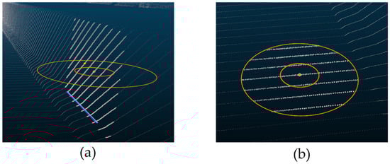
Figure 64.
Representing the importance of setting the location of the search area to detect the road boundary. (
a
) The error of detecting the edge occurs because the search area (the large orange circle in (
a
)) is not adjacent to the road surface. (
b
) None of the edges are identified due to the search area (the large orange circle in (
b)) only including the road surface.
)) only including the road surface.
The plane fitted to the lowest points is defined by calculating the normal vectors of the points. Each point has a position in the point cloud data (x, y, z). Each point is collected, which together form a group of points to represent the appearance of an object. The higher the density of the point group, the more detailed the shape that can be expressed. Moreover, the point cloud data acquired from ground MMS surveys have an average precision of 2 cm; therefore, points with 2 cm errors along the y-axis were also included to fit the plane. In point cloud data, the edge of the road plane can be extracted by calculating the normal vectors based on the coordinates of each point and fitting the points to a plane. The normal vector is perpendicular to the plane. Assuming that there are three points (P1, P2, and P3) on the plane, the normal vector (N) to the plane can be obtained by calculating the cross product of the two vectors 𝑃2−𝑃1 and 𝑃3−𝑃1 (Figure 75).

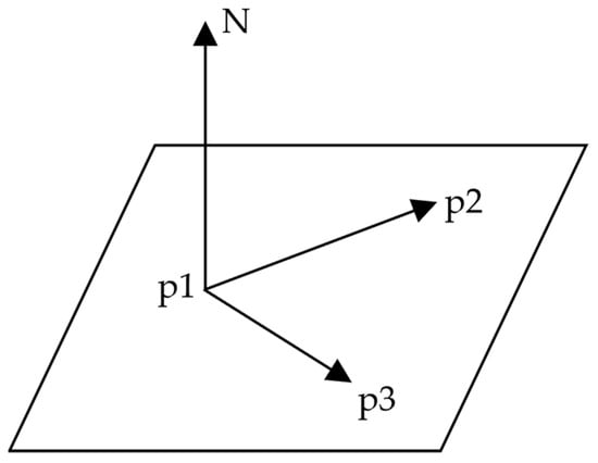
Figure 75.
The cross product of two vectors for a normal vector (
N).
).
The normal vector is calculated with Equation (1) or Equation (2).


An algorithm to calculate a normal vector is described as Algorithm 1.
| Algorithm 1: Calculating a normal vector (N) |
| 1 Input: point p1, point p2, point Bp3 2 𝐴,OBB 𝐵,noOutput: normal vector N(x, ry, z) 3 vector mal Vector ):𝑢= 2 for(𝑖 = 0; 𝑖 < 𝐴.𝐴𝑙𝑙𝑁𝑜𝑑𝑒𝑠𝑝0–𝑝1 4 vector 𝑣=𝑝0–𝑝2 5 6 //Calculating a plane to find normal vector 7 vector N = crossProduct(u, v) //perform cross product of two lines on the plane 8 9 If vectorSize(N) > 0 10 ; 𝑖++): 3 𝑡= 𝐴.𝑉.𝑁𝑜𝑑𝑒[𝑖] 4 𝑑𝑀m_n = normalize(N) // after normalization, assign it into a new variable m_n 11 12 𝑖𝑛 = t 5 𝑑𝑀𝑎𝑥 = t 6 // calculate the length between nodes 7 for (c = 1; c < 𝐴.𝑉.𝑁𝑜𝑑𝑒𝑠[𝑖]; c++): 8 𝑡 = (𝑡 + 𝐴.𝑉.𝑁𝑜𝑑𝑒𝑠[𝑖]𝑚_𝑑=𝑚_𝑛∗𝐴 // the distance between the origin point and the plane 13 End 14 15 //Calculating normal vector using orientation values 16 ) / 2 9 if (𝑡<𝑑𝑀𝑖𝑛): 10 𝑑𝑀𝑖𝑛=𝑡 11 elseif (𝑡>𝑑𝑀𝑎𝑥𝑙): 12 𝑑𝑀𝑎𝑥=𝑡𝑒𝑛𝑔𝑡ℎ=𝑠𝑞𝑟𝑡(𝑥∗𝑥+𝑦∗𝑦+𝑧∗𝑧) 17 𝑥=𝑥/𝑙𝑒𝑛𝑔𝑡ℎ 18 𝑦=𝑦/𝑙𝑒𝑛𝑔𝑡ℎ 19 𝑧=𝑧/𝑙𝑒𝑛𝑔𝑡ℎ |
As mentioned above, the normal vectors of the points were calculated (Figure 86a), and points whose normal vectors were nearly 90° (approximately over 85°) were fitted to a plane by applying the k-NN clustering algorithm (Figure 86b). The boundary line is formed by connecting the edge’s endpoints where the plane from the points ends. The points on the edge of the plane were connected, creating a reference line aligned with the u-axis of the OBB (Figure 86c). This method applied the width of the OBB, which was aligned with the v-axis up to 50 cm. When the radius of the search area is 50 cm, the length of the edge can be generated to be utile 1 m. However, to create a rectangular OBB for directionality, wthe researchers applied an OBB width of up to 50 cm.
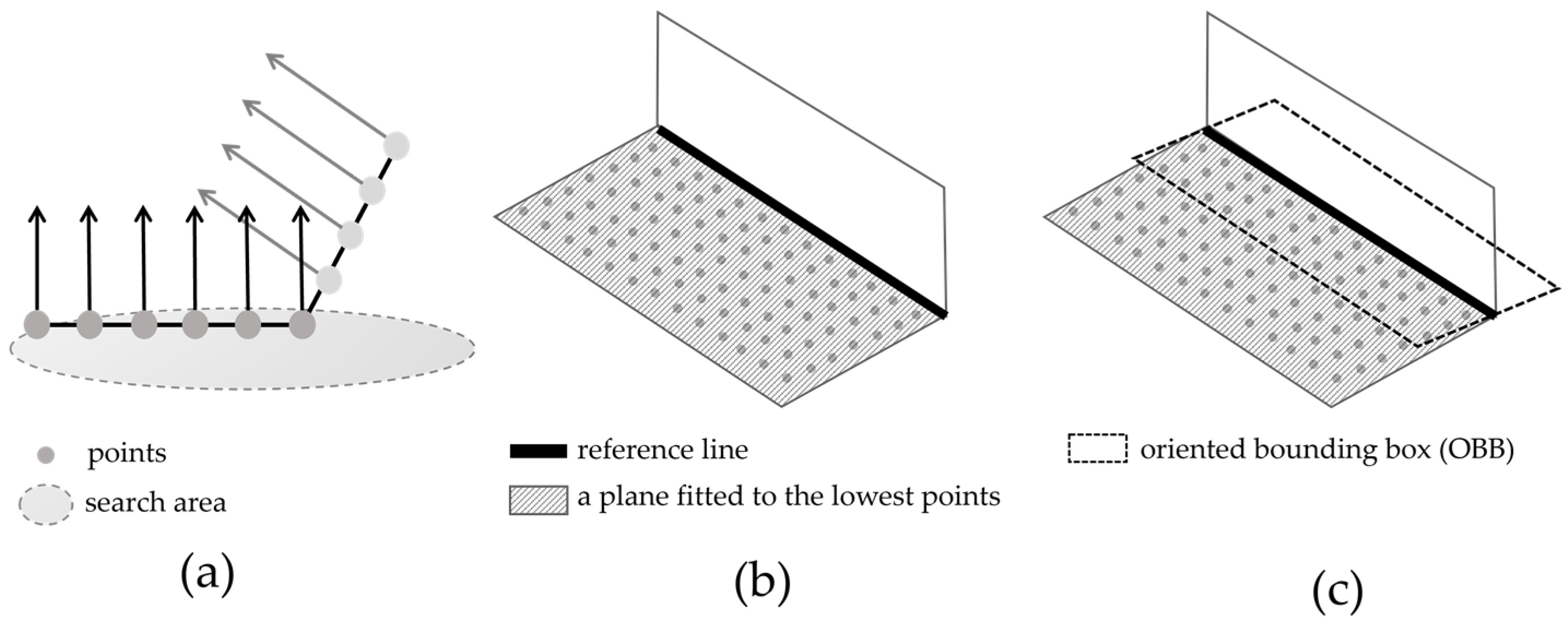
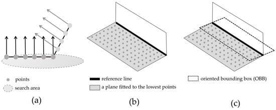
Figure 86.
Generating oriented bounding box (OBB) of road boundaries. (
a
) Calculating normal vectors in the search area and selecting parts of them over 85 degrees. (
b
) Making a plane using the k-NN algorithm and generating a reference line (the black solid line in (
b
)) at the boundary. (
c
) Generating OBB (the black dotted rectangle in (
c)) based on the reference line.
)) based on the reference line.
2. Creating Oriented Bounding Box of Edge Markings and Linear Road Markings Using Intensity Value
The point cloud data store the intensity and position values. In the point cloud data, the intensity values are stored as a short (unsigned short) type, and the value ranges from 0 to 255, where the higher the number, the higher the reflection rate. Linear road markings, which are edge and lane markings, are more likely to have a higher intensity than the surrounding environment because of the glass beads. Therefore, using intensity values, this study classifies linear road markings from point cloud data.
A range of intensity values must be established to distinguish between linear road markings. However, the intensity values are distributed depending on the measurement environment, such as weather, sunlight, and shadows. This means the intensity distribution can differ for each measurement even if the same area is resurveyed. Therefore, the intensity corresponding to linear road markings should be checked and set to include its value. After setting the range of intensity values that classified the linear road markings and road surfaces, the points of the extracted linear road markings were combined to determine the fitted plane (Figure 97).

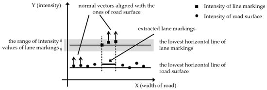
Figure 97. Extracting road lane area based on the normal vector of the plane.
Extracting road lane area based on the normal vector of the plane.
Similar to the generation of the OBB of the road boundaries in the previous section, the points included in the search area are selected first. Subsequently, a reference line to generate the OBB of linear road markings was determined by connecting the endpoints of the point group included in the intensity value range. The centerline of the corresponding road markings was set as a reference line aligned with the u-axis of the OBB, and the width was defined as the width of the extracted linear road markings, which was 20 cm (Figure 108a). The search area, including the road marking areas, must be located to generate the OBB (Figure 108b). Even if the search area included the marking area, linear road markings with intensity values outside the set range cannot be detected, as shown in Figure 108c. None of the markings are identified if the search area excludes the marking area (Figure 108d).
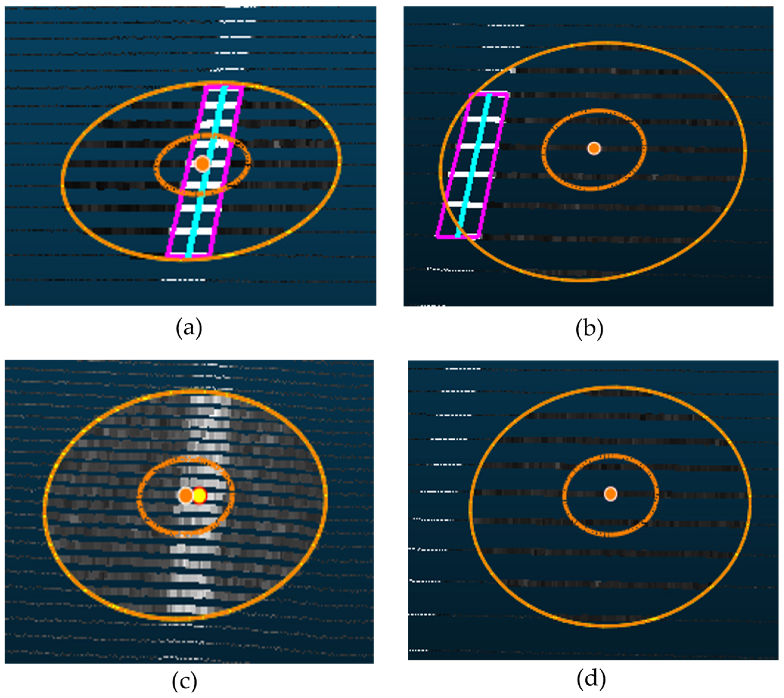

Figure 108.
(
a
) The search area (the orange circles in (
a
,
b
)) detects linear road markings using intensity values. The center line (the sky-blue line in (
a
,
b
)) of the extracted area is a reference line of OBB, and the width is 20 cm, which determines an OBB (the pink rectangle in (
a
,
b
)). (
b
) The search area can detect the linear road markings by including the width of it. (
c
) The linear road markings whose intensity values are out of the range fail to be identified. (
d) The search area cannot find linear road markings due to the exclusion of the markings area.
) The search area cannot find linear road markings due to the exclusion of the markings area.
3. Automatic Extraction of Road Boundary and Road Markings Using Collision-Detection Algorithm
Using the generated OBBs for the road boundaries and linear road markings, linear data can be automatically extracted by setting a search radius based on these data. The OBB collision-detection algorithm is used to extract the linear data automatically. The OBB collision-detection algorithm operates based on the separating axis theorem (SAT), in which polygons are projected onto one axis and recognized as colliding objects when the projection sections overlap. In this study, the OBB was a rectangle parallel to the road-driving direction.
If an OBB rectangle is created, the OBB collision-detection algorithm connects the centerline of the conflicting OBB to build linear data based on the object. The separation axis of the figure used for applying the OBB collision-detection algorithm should apply a normal vector from the reference axis. In this study, the direction of the road was defined as the reference axis for extracting the road boundaries and lanes. If the road direction was set to that of the separation axis, the following process calculated the collision. The normal vector of the reference axis was used to check for collisions (Zhang et al. (2019) [30][2]), as shown in Figure 119: if the distance between the center point of 𝑂𝐵𝐵 𝐴 and that of 𝑂𝐵𝐵 𝐵 is defined as 𝑇, 𝑇 is a vector with directionality. The value projected from the vector with directionality becomes 𝑇·𝐿 (Figure 119). In addition, if the sum of the length of 𝑃𝐴 projecting the longest point from the center point of 𝐴 to the direction of 𝐵 and the length of 𝑃𝐵 projecting the long point from the center point of 𝐵 to the direction of A is greater than 𝑇·𝐿, a collision has occurred (Figure 119).
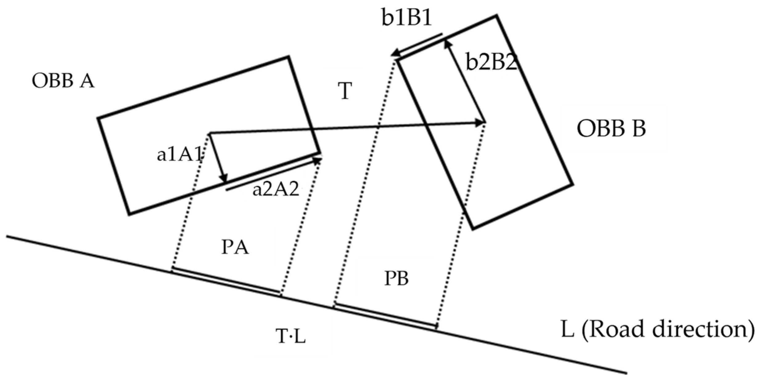
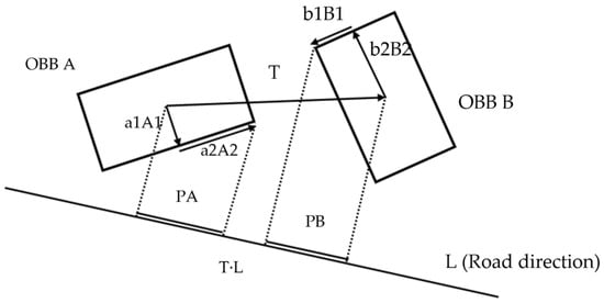
Figure 119. Representing separating axis theorem (SAT).
Representing separating axis theorem (SAT).
The collision calculation method of the separation axis theory is defined in Equations (3)–(5):


To automatically extract the linear data, the reference data to which the first acquired OBB is applied are used to check whether a line connects forward and backward. The search method obtains the range’s start- and endpoint groups by applying a search interval. Because the road may not be horizontal, an OBB was generated by applying a height equal to the search width. Subsequently, the OBB was generated at a position corresponding to the forward and backward intervals. The OBB is connected to the corresponding OBB and reference data to connect the lines (Figure 120).

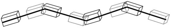
Figure 120. Creating linear data with OBB centerline connections.
Creating linear data with OBB centerline connections.
The pseudocode for the OBB collision-detection algorithm is as follows (Algorithm 2).
| Algorithm 2: Overlapped OBB collision detection algorithm |
| 1 function OverlapOBB (OB 13 // check the length is in the range between dMin and dMax 14 if ((𝑑𝑀𝑖𝑛>𝑡)||(𝑑𝑀𝑎𝑥<𝑡): 15 // The OBBs are not overlapped 16 return false 17 return true |
The two elements of the initial settings were search intervals: search length and width. The proper setting of search intervals is essential because the proposed automatic extraction method can be applied to straight and curved roads. Therefore, the search length and width are the parameters of this method based on the conditions of the applied site, which should be applied differently depending on the shape of the road. For example, highly accurate linear data can be extracted from straight roads by increasing the search length and applying a narrow search width. The search length should be shortened for curved roads, and a wide search width should be applied. The procedure for generating linear data by applying the OBB collision-detection algorithm is shown in Figure 113.

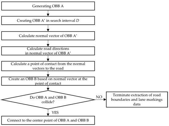
Figure 113. The procedure of the OBB collision-detection algorithm to extract road boundaries and linear road markings.
The procedure of the OBB collision-detection algorithm to extract road boundaries and linear road markings.
𝑂𝐵𝐵 𝐴 generated as reference data was moved using a search length based on the road direction to generate 𝑂𝐵𝐵𝐴′ in the corresponding direction. The normal vector is then obtained from the direction of 𝑂𝐵𝐵 𝐴′, and the point at which the normal vector meets the direction of the road is obtained. After that, the normal vector is calculated at the corresponding point, and 𝑂𝐵𝐵 𝐵 is generated based on the road direction and normal vector. Subsequently, 𝑂𝐵𝐵 𝐴′ and 𝑂𝐵𝐵 𝐵 were inspected for collisions using the OBB collision-detection algorithm (Figure 142a). Collision detection was performed in the above order. When a collision was detected, linear data were generated by connecting the center points of 𝑂𝐵𝐵 𝐴 and 𝑂𝐵𝐵 𝐵 (Figure 142b).

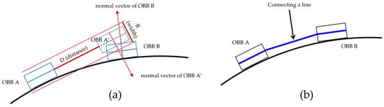
Figure 142.
(
a
) Applying the OBB collision-detection algorithm and (
b) connecting the center line of OBB A and OBB B.
) connecting the center line of OBB A and OBB B.
References
- Siwei, H.; Baolong, L. Review of Bounding Box Algorithm Based on 3D Point Cloud. Int. J. Adv. Netw. Monit. Control. 2021, 6, 18–23.
- Zhang, X.; Liu, J.; Liu, Z.; Zhang, L.; Qin, X.; Zhang, R.; Liu, X.; Wei, J. Collision Detection Based on OBB Simplified Modeling. J. Phys. Conf. Ser. 2019, 1213, 042079.
More