+1 credit
| Version | Summary | Created by | Modification | Content Size | Created at | Operation |
|---|---|---|---|---|---|---|
| 1 | Alexei Finkelstein | + 6867 word(s) | 6867 | 2021-04-06 10:15:42 | | | |
| 2 | Catherine Yang | + 61 word(s) | 6928 | 2021-04-09 03:55:08 | | | | |
| 3 | Catherine Yang | -96 word(s) | 6832 | 2021-04-09 11:50:49 | | | | |
| 4 | Catherine Yang | Meta information modification | 6832 | 2021-04-15 05:20:58 | | | | |
| 5 | Alexei V. Finkelstein | Meta information modification | 6832 | 2021-04-21 15:06:53 | | | | |
| 6 | Alexei V. Finkelstein | Meta information modification | 6832 | 2021-04-21 15:09:00 | | | | |
| 7 | Alexei V. Finkelstein | + 75 word(s) | 6907 | 2021-04-21 16:15:17 | | |
Video Upload Options
Protein folding is a process that converts the unfolded, disordered protein chain into a chain having a definite, unique three-dimensional structure.
Preface
Currently, the term "protein folding problem" has two meanings, one emphasizing the process, the other the result. The former (sometimes called "the protein folding problem of the first order") implies the answer to the question of how the protein chain chooses, in minutes, its unique structure among a giant number of others; the latter (sometimes called "the protein folding problem of the second order") implies the answer to the question of what structure will be attained by the protein chain of a certain amino acid sequence. For a long time, these two problems were considered as one, assuming that once "how" were solved, "what" would be solved right away. However, now it is clear that these are two different problems, because they have been solved by two quite different methods. The problem of "what" has been very recently solved by bioinformatics with the aid of neural networks and artificial intelligence [Senior et al., 2019, 2020; Yang et al., 2020]. This topic needs to be described in a separate Entry of Encyclopedia. The problem of "how" has been solved by physics. The aim of the article below is to outline the principal moments of this solution.
1. Introduction
The ability of proteins to fold spontaneously puzzled protein science for a long time (see, e.g., [Anfinsen & Scheraga, 1975; Jackson, 1998; Fersht, 2000; Grantcharova et al., 2001; Robson & Vaithilingam, 2008; Dill & MacCallum, 2012; Wang et al., 2012; Wolynes, 2015; Finkelstein & Ptitsyn, 2016]).
As known, in living cells, gene-encoded protein chains are synthesized by special molecular machines, called ribosomes. To perform its unique biological function, the protein chain has to obtain its unique ("native") three-dimensional (3D) structure.
This phenomenon is called "protein folding".
Its importance for protein functioning was recognized in the 1950s [Anfinsen, 1959], followed by the finding that protein folding can occur not only in vivo but also in vitro [Anfinsen et al., 1961].
2. Experimental studies of protein folding
Since it is rather difficult to follow a change in the structure of a nascent protein chain against the background of many other molecules in a living cell, the investigation of protein folding started with in vitro experiments on the folding of water-soluble molecules of globular proteins.
However, it makes sense to begin this paper with a short overview of comparatively recent results on the folding that occurs in the course of protein biosynthesis on ribosomes.
The first studies were carried out on large proteins. They showed that these start to fold before their biosynthesis has been completed: the first synthetized (N-terminal) immunoglobulin domain folds when the whole chain has not been synthesized yet [Isenman et al., 1979]; the luciferase protein starts to work immediately upon completion of the chain biosynthesis [Kolb et al., 1994]; and the globin chain can bind to the heme when a bit more than its half has been synthesized by the ribosome [Komar et al., 1997] (though it is hard to say whether structuring of this half-made chain occurred before the heme-binding or resulted from it). Anyway, these data suggest that the in vivo protein chain folding starts just on the ribosome and that this co-translational process differs from the discussed below in vitro folding ("renaturation") of the entire protein chain.
However, more up-to-date experiments on co-translational structure acquisition by small nascent proteins (monitored by 15N, 13C NMR, and FRET) have shown that “polypeptides [at a ribosome] remain unstructured during elongation but fold into a compact, native-like structure when the entire sequence is available” [Eichmann et al., 2010]; “… folding [occurs] immediately after the emergence of the full domain sequence” [Han et al., 2012]; “… co-translational folding … proceeds through a compact, non-native conformation [i.e., something molten globule-like] … [and] rearranges into a native-like structure immediately after the full domain sequence has emerged from the ribosome” [Holtkamp et al., 2015].
Thus, there is no fundamental difference between the in vivo and in vitro folding, at least for small proteins, though some details of the on-ribosome and in vitro folding pathways can differ. In both cases, native structures emerge only when the entire sequence of a protein domain has been synthesized (it should be noted that truncated protein chains do not refold and remain compact but disordered in vitro [Flanagan et al., 1992]).
The discovery of chaperones, the cell’s troubleshooters [Ellis & Hartl, 1999], again aroused numerous suggestions that the in vivo and in vitro protein folding may be quite different, because chaperones may have a foldase/unfoldase activity (see, e.g., [Libich et al., 2015] and references therein). However, the analysis of data presented in [Libich et al., 2015] reveals that the most studied chaperone (GroEL) does not speed up the overall folding process [Marchenko et al., 2015]. This corroborates the conclusion that GroEL serves as an auxiliary transient trap that binds excess unfolded protein chains, thus preventing them from irreversible aggregation [Marchenkov et al., 2004; Marchenko et al., 2009].
Thus, the self-organization of protein structures (which in the case of in vitro folding of water-soluble globular proteins is unassisted by other biomolecules) captures the main peculiarities of the protein folding phenomenon. This means that all the information necessary to build up the 3D structure of a protein is inscribed in its amino acid sequence (this was Anfinsen's "thermodynamic hypothesis").
The study of self-organization has shown that an unfolded protein chain can spontaneously, "by itself", fold into its unique native 3D structure [Anfinsen et al., 1961; Anfinsen, 1973]. In Anfinsen's experiment, the enzyme ribonuclease A unfolded in the presence of urea and a thiol reagent, and with these agents removed, the enzyme spontaneously refolded, recovering its structure (as shown by correct restoration of all four S-S bonds) and function. However, as it has been recently found by David Eisenberg [2018], "essentially the same experiment had been performed earlier by a medical student [Lisa A. Steiner] at Yale, but neither [she nor] her research supervisor nor her department chair thought it particularly significant, and her work was not published". "Why did this transformative result lay hidden in her thesis?" asked Eisenberg, and answered: "She had the answer to a hugely important question, but that question had not yet been posed" because then (in the mid-1950s) it had not yet been elucidated "how biological information passes from the genome to proteins".
3. The protein folding problem
In the course of self-organization, the protein chain has to find its native (and seemingly the most stable) fold among zillions of others (Fig. 1) within only minutes given by a cell for its folding.
Indeed, the number of alternatives is vast [Levinthal, 1968, 1969]: it is at least 2100 but more likely 3100 or even 10100 (or 100100) for a 100-residue chain, because at least 2 ("right" and "wrong") but more likely 3 (α, β, "coil") or ≈10 (Privalov's [1979] experimental estimate), or even 100 [Levinthal, 1969] conformations are possible for each residue.
Since the chain cannot pass from one conformation to another faster than within a picosecond (the time of a thermal vibration), the exhaustive search would take at least ~2100 picoseconds (but more likely 3100, or even 10100, or 100100), that is, ~1010 (or 1025, or even 1080, or 10180) years. And it looks like the sampling has to be exhaustive because the protein “feels” that it has come to the stable structure only when it hits it precisely, while even a 1Å deviation can strongly increase the chain energy in the closely packed globule.
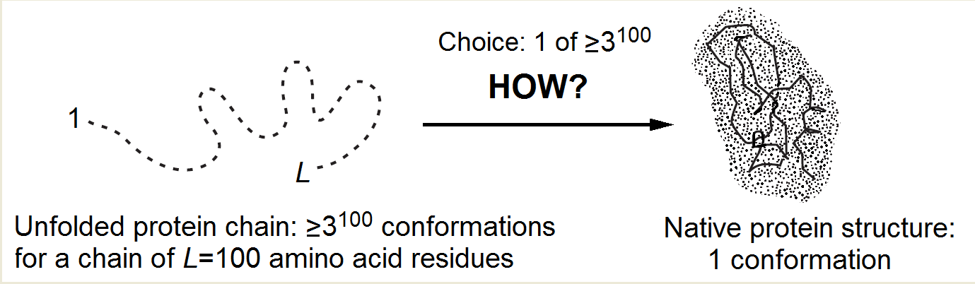
Figure 1. The Levinthal's choice problem. The choice of the native structure can be determined either by the folding process (Levinthal's "kinetic hypothesis") or by the enhanced native fold stability (Anfinsen's "thermodynamic hypothesis").
The main protein folding puzzle is why the native protein structure is found within minutes rather than within "Levinthal's" ~1010 or more years (that is, within ~1016 or more minutes)! This reduction of the folding process by 10 000 000 000 000 000 (!) times (compared to iterating over all structures) must be always kept in mind without distracting to dead-end considerations that promise, say, 1 000- or 1 000 000-fold acceleration of the process.
How can the protein chain choose, in minutes, its native structure among a giant number of others, asked Levinthal [1968; 1969] (who first noticed this paradox), and answered: It seems that the protein folding follows some specific fast pathway, and the native fold is simply the end of this pathway, no matter if it is the most stable chain fold or not (this was Levinthal's "kinetic hypothesis"). In other words, Levinthal suggested that the native protein structure is determined by kinetics rather than stability and corresponds to the easily accessible local free energy minimum rather than the global one.
However, computer experiments with lattice models of protein chains strongly suggest that the chains fold to their most stable structure, i.e., that the "native protein structure" is the lowest-energy one, and protein folding is under thermodynamic rather than kinetic control [Šali et al., 1994; Abkevich et al., 1994].
Nevertheless, most of the proposed and widely discussed hypotheses on protein folding were based on the "kinetic" (rather than "thermodynamic") "control assumption".
In particular, ahead of Levinthal, Phillips [1966] proposed that the protein folding nucleus is formed near the N-end of the nascent protein chain, and the remaining chain wraps around it. Meanwhile, the successful in vitro folding of many single-domain proteins and protein domains does not begin from the N-end [Goldenberg & Creighton, 1983; Grantcharova et al., 1998; Lappalainen et al., 2008].
Wetlaufer [1973] hypothesized the formation of the folding nucleus by adjacent residues of the protein chain but in vitro experiments have shown that this is not always so [Fulton et al., 1999; Wensley et al., 2009].
Ptitsyn [1973] proposed a model of hierarchical folding, i.e., a stepwise involvement of different interactions and the formation of different folding intermediate states.
More recently, various “folding funnel” models [Leopold et al., 1992; Wolynes et al., 1995; Dill & Chan, 1997; Bicout & Szabo, 2000; Wang et al., 2012] have become popular for illustrating and describing the reason for the speedy folding processes.
The difficulty of the "kinetics vs stability" problem is that it hardly can be solved by a direct experiment. Indeed, suppose that a protein has some structure that is more stable than the native one. How can we find it if the protein does not do so itself? Shall we wait for ~1010 (or even ~10180) years?
On the other hand, the question as to whether the protein structure is controlled by kinetics or stability arises again and again in solving practical problems of protein physics, engineering, and design. For example, when predicting the protein structure from its sequence, what should we look for? The most stable or the most rapidly folding structure? When designing a de novo protein, should we maximize the stability of the desired fold or create a rapid pathway to this fold?
However, is there a contradiction between “the most stable” and the “rapidly folding” structure? Maybe, the stable structure automatically forms a focus for the “rapid” folding pathways, and therefore it is automatically capable of fast-folding?
4. The major thermodynamic peculiarities of protein folding
Before considering these questions, i.e., before considering the kinetic aspects of protein folding, let us recall some basic experimental facts concerning protein thermodynamics (as usual, we will consider single-domain water-soluble globular proteins only, i.e., chains of ~100 residues). These facts will help us understand what chains and folding conditions we have to consider. The facts are as follows:
- Nearly all observations show that native states of single-domain water-soluble globular proteins behave as the lowest-energy folds [Tanford, 1968; Privalov, 1979; Fersht. 1999]. However, there is at least one exception: a large (≈400 residues) protein serpin first obtains the "native" (that is, "working") structure, works for half an hour, and then acquires another, non-working but more stable structure [Tsutsui et al., 2012].
- The denatured state of proteins, at least that of small proteins treated with a strong denaturant, is usually an unfolded random coil (while the temperature-denatured state can be a compact molten globule) [Tanford, 1968; Ptitsyn, 1995].
- Protein unfolding is reversible [Anfinsen, 1973]; moreover, the denatured and native states of a protein can be in a kinetic equilibrium [Creighton, 1978]; there is an “all-or-none” transition between them [Privalov, 1979]. The latter means that only two states of the protein molecule, native and denatured, are present (close to the mid-point of the folding-unfolding equilibrium) in a visible quantity, while all others, "semi-native" or misfolded, are virtually absent. (Notes: (i) the “all-or-none” transition makes the protein function reliable: like a light bulb, the protein either works or not; (ii) the physical theory shows that such a transition requires the amino acid sequence that provides a large "energy gap" between the most stable structure and the bulk of misfolded ones [Shakhnovich & Gutin, 1990; Gutin & Shakhnovich, 1993; Šali et al., 1994; Galzitskaya & Finkelstein, 1995; Shakhnovich, 2006]).
- Even under normal physiological conditions, only a few kilocalories per mole [Privalov, 1979] differ the native (i.e., the lowest-energy) state of a protein from its unfolded (i.e., the highest-entropy) state (and these two states have equal stabilities at mid-transition, naturally).
(For the below theoretical analysis, it is essential to note that (i) as is customary in the literature on this subject, the term “entropy” as applied to protein folding means conformational entropy of the chain without solvent entropy; (ii) accordingly, the term “energy” actually implies “free energy of interactions” (often called the “mean force potential”), so that hydrophobic and other solvent-mediated forces, with all their solvent entropy [Tanford, 1968], come within “energy”. This terminology is commonly used to concentrate on the main problem of sampling the protein chain conformations.)
The above-mentioned “all-or-none” transition means that the native (N) and denatured (U) states are separated by a high free-energy barrier. It is the height of this barrier that limits the rate of this transition, and just this height is to be estimated to solve Levinthal's paradox.
5. The major kinetic peculiarities of protein folding
The “kinetic control” hypothesis initiated very intensive studies of protein folding intermediates.
It was clear almost from the very beginning that the stable intermediates are not obligatory for folding, since the protein can also fold near the mid-point of equilibrium between the native and denatured states (Fig. 2) [Segava & Sugihara, 1984], where the transition is of the “all-or-none” type [Privalov, 1979], which excludes any stable intermediates.
The obtained basic experimental facts on protein folding kinetics are as follows:
- The protein folding unit is a domain. This has been shown by two groups of evidence: (i) separate domains are usually capable of folding into the correct structure [Petsko & Ringe, 2004]; (ii) single-domain proteins usually cannot fold when as few as 10 of their C- (or N-) terminal amino acids are deleted [Flanagan et al., 1992; Neira & Fersht, 1999a,b].
- Folding of some proteins proceeds as a two-state process without any accumulating intermediates (when only two states, the native fold and the coil are observable [Matouschek et al., 1990; Fersht, 1999]), whereas the folding of other single-domain proteins, mostly larger ones (and especially the folding occurring far from the equilibrium mid-point) exhibit multi-state kinetics where molten and/or pre-molten globules serve as the folding intermediates [Dolgikh et al., 1984; Ptitsyn, 1995; Fersht, 1999].
- When the folding process proceeds via the folding intermediates, the rate-limiting step immediately precedes the native state formation and corresponds to transition from the rather dense molten globule to the native structure [Dolgikh et al., 1984].
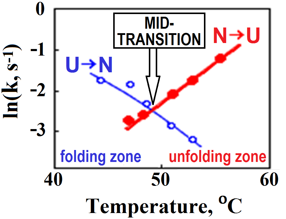
Figure 2. Rates (k) of lysozyme re- and denaturation vs temperature. The mid-transition point is where the rates of renaturation (U→N) and denaturation (N→U transition) are equal, i.e., where the curves intersect. The plot is adapted from [Segava & Sugihara, 1984]. Note that folding at physiological temperatures of ≈40oC is only ~10-fold faster than folding at the mid-transition point. The similar in value but the opposite slopes of the U→N and N→U lines indicate that the transition state is intermediate in properties between the native and denatured states.
6. Understanding of the protein folding times
To begin with, it is not out of place considering whether the “Levinthal’s paradox” is a paradox indeed. Bryngelson & Wolynes [1989] mentioned that this “paradox” is based on the absolutely flat (and therefore unrealistic) “golf course” model of the protein potential energy surface (Fig. 3a), and somewhat later Leopold et al. [1992], following the line of Go & Abe [1981], considered more realistic (tilted and biased to the protein native structure) energy surfaces and introduced the “folding funnels” (Fig. 3b), which seemingly eliminate the “paradox”.
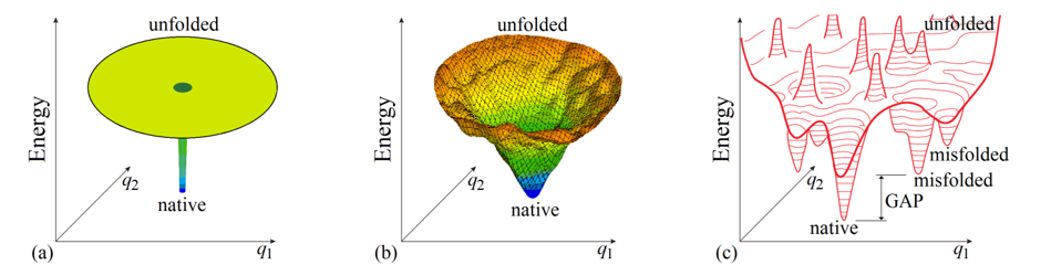
Figure 3. Schematic illustration of basic models of the energy landscapes of protein chains. (a) The “Levinthal's golf course model". (b) The “funnel” model; the funnel is centered in the lowest-energy (“native”) structure. (c) The potential energy landscape of a protein chain in more detail with bumps and wells, the deepest of which ("native") is by many kBTmelt (where kB is Boltzmann's constant and Tmelt is protein melting temperature) deeper than the others: this energy GAP between the global and other energy minima is necessary to provide the “all-or-none” type of decay of the stable protein structure [Shakhnovich & Gutin, 1990]. Only two coordinates (q1 and q2) can be shown in the figures, while the protein chain conformation is determined by hundreds of coordinates.
Various “folding funnel” models became popular for explaining and illustrating protein folding [Wolynes et al., 1995; Karplus, 1997; Nölting, 2010; Wolynes, 2015]. In the funnel, the lowest-energy structure (formed by a set of the most powerful interactions) is the center surrounded by higher-energy structures containing only a part of these powerful interactions. The “energy funnels” may appear not perfectly smooth due to some "frustrations" [Bryngelson & Wolynes, 1987, i.e., contradictions between optimal interactions for different links of a heteropolymer forming the protein globule, but a stable protein structure is distinguished by minimal frustrations (that is, most of its elements enhance the native fold stability) [Bryngelson & Wolynes, 1987, 1989; Bryngelson et al., 1995; Finkelstein et al., 1995]. The “energy funnel” can channel the protein chain towards the single lowest-energy structure, thereby apparently preventing “Levinthal’s” sampling of all conformations.
This would be so provided there were only energy and no entropy, which (if temperature >0oK) opposes the chain movement towards the single structure, even though corresponding to the global energy minimum.
But protein folding occurs in liquid water, at temperatures >273oK, where the entropy term is big, and, moreover, the folding proximity to the mid-transition point (Fig. 2) makes the entropy term compensate for the folding energy.
The mid-transition point fits the best to analyze Levinthal’s paradox (though in the "strongly folding conditions" the folding can be, say, 1 000-fold faster – but this is infinitely less than the puzzling 10 000 000 000 000 000-fold acceleration of the folding process compared to iterating over all structures).
At the mid-transition point, the protein chain has two equally stable low-free-energy states (denatured, often to the random coil, and natively folded) which are separated by a free energy barrier providing the all-or-none transition between them [Privalov, 1979], and the free energy landscape is "volcano-shaped" [Rollins & Dill, 2014] (Fig. 4).
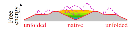
Figure 4. This purely illustrative drawing shows how entropy converts the energy funnel (Fig. 3b) into a "volcano-shaped" free-energy folding landscape with a barrier on any pathway leading from unfolded conformations to the native fold. The smooth free energy landscape corresponds to compact semi-folded intermediate structures; the rocks (denoted by dotted lines) present the high-energy non-compact semi-folded intermediate structures and intermediate structures with high-energy bumps (see Fig. 3c). More accurate but less beautiful scheme of the free-energy landscape is shown in Fig. 2 in [Galzitskaya & Finkelstein, 1999].
Thus, any pathway from the unfolded state to the native one first goes uphill in free energy, and only then, in the vicinity of the native state, after passing the free energy barrier (i.e., the crater edge), the "free-energy funnel" starts working and pulls the chain downhill to the native state.
To have a rapid transition from the coil to the native state, the free energy barrier created by the volcano must be not high: according to the conventional transition state theory [Eyring 1935; Pauling, 1970; Emanuel & Knorre, 1984], the time of overcoming the barrier is estimated as
TIME ≈ τ × exp(+∆F#/kBT) (1)
where τ is the time of a step from the barrier onwards, and ∆F# is the height of the free energy barrier (that is, the free energy of the folding nucleus).
It should be noted that protein folding is a multistep process [Finkelstein & Ptitsyn, 2002], and the traditional steady state theory is not very accurate when applied to multistep processes, including protein folding [Djikaev & Ruckenstein, 2016] and phase transitions in general [Ruckenstein & Berim, 2016]. However, this relatively small error mainly concerns [Finkelstein, 2015; Ruckenstein & Berim, 2016] to the estimate of the pre-exponential factor (τ in equation (1)), which is of secondary importance compared to the main term (exponent in equation (1) that accounts for the transition state free energy).
Because not any type of energy funnel provides a low volcano height, not any energy funnel per se can resolve Levinthal’s paradox. Strict analysis [Bogatyreva & Finkelstein, 2001] of the straightforwardly presented funnel models [Zwanzig et al, 1992; Bicout & Szabo, 2000] corresponding to the uniform condensation of the chain (previously considered by Shakhnovich & Finkelstein [1989]) shows that close to the mid-transition point such funnels cannot simultaneously explain both major features observed in protein folding: (i) its non-astronomical time and (ii) the "all-or-none" type of transition. By the way, the stepwise folding mechanism [Ptitsyn, 1973] also cannot [Finkelstein, 2002] simultaneously explain both of these, and hence, cannot resolve Levinthal's paradox.
The basic solution of the paradox is provided by funnels of a special type providing separation of folded and unfolded phases [Finkelstein & Badretdinov, 1997a, b] within the folding chain. (Which, as it was later mentioned in a review by Wolynes [1997], resembles the "capillarity in the nucleation" in the first-order phase transitions. The separation of the folded and unfolded phases in protein folding is seen in later computer simulations by Shaw et al. [2010]).
The optimal pathway of folding can be outlined using the optimal pathway of unfolding (which can be found much easier) because, according to the well-known detailed balance law [Landau & Lifshitz, 1980], the direct and reverse reactions follow the same pathway and have equal rates when both end-states have equal stability (otherwise, i.e., if the pathways for  and
and  reactions were different, the result would be a permanent circular flow
  (generating a perpetual motion machine of the second kind), which contradicts to the second law of thermodynamics).
As for a good unfolding pathway, one can easily figure out that this can be a sequential unfolding pathway passing through the least unstable semi-unfolded states, i.e., those where the compact globular phase is separated from the unfolded one by a relatively small boundary (Fig. 5) [Finkelstein & Badretdinov, 1997a, b; Galzitskaya & Finkelstein, 1999; Garbuzynskiy et al., 2013]. (To resolve Levinthal's paradox, it is not necessary to prove that this is the best possible pathway; it is enough to prove that this pathway resolves the paradox because any additional pathway will only accelerate the process. Imagine two pools, full of water and empty, with water leaking from one to the other through cracks in the wall between them; when the cracks cannot absorb all the water – which is prohibited by the all-or-none transition – each additional crack accelerates filling of the empty pool.)
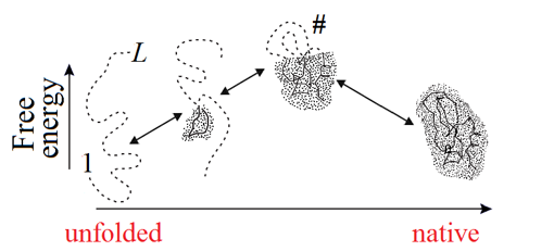
Figure 5. Schematic illustration of the sequential folding/unfolding pathway of a globule with compact semi-folded intermediates. At each step of sequential unfolding, one residue leaves the native-like part of the globule (shaded) and turns into a coil (shown by a dashed line). The highest-free-energy intermediate (the folding nucleus corresponding to the transition state, denoted as #) has the largest (on the pathway) interface of the globular and unfolded phases. Its globular part covers about half of the chain. Adapted from [Finkelstein & Badretdinov, 1997a, b].
In a simplified form (for details, see [Finkelstein & Badretdinov, 1997a, b; 1998; Garbuzynskiy et al., 2013]), the resulting free energy barrier is estimated as follows.
When the free energies of the folded and unfolded phases are equal (i.e., in the mid-transition ambient conditions), the free energy of a semi-folded structure depends only on the interface between the two phases. The largest unavoidable interface corresponds to the intermediate that looks like a half of the native globule (Fig. 5) and has ≈L2/3 residues at the interface (assuming the most compact spherical shape of the native globule; for an oblate or oblong globule, the largest unavoidable interface can be a little less).
Thus, the transition state free energy is proportional not to the number L of the chain residues (as Levinthal’s estimate implies), but to L2/3 only.
The energy constituent ΔE# of the barrier free energy ΔF# results from interactions lost by the interface residues; it is about 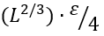 , where ε ≈ 1.3 kcal/mol ≈ 2kBTmel is the average latent heat of protein melting per residue [Privalov, 1979] (this is the first empirical parameter used by the theory), and ≈1/4 is, roughly, the fraction of interactions lost by an interface residue. Thus,
![]() (2)
(2)
The entropy constituent ΔS# of the barrier free energy ΔF# is caused by entropy lost by closed loops protruding from the globular into the unfolded phase (note that the second folding intermediate, denoted as # in Fig. 5, contains two closed loops, and the first folding intermediate in Fig. 5 contains no closed loops).
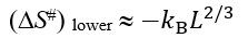
When the shape of the native protein fold and especially the shape of the chain fold in the transition state are not known, the closed-loops-connected ΔS# value (which is ≤0) can only be estimated from above and below. The upper limit of ΔS# is zero (when the interface contains no closed loops). The lower limit of ΔS# is about
 (3)
(3)
Here, ![]() is the maximal expected number of loops protruding from the maximal (containing
is the maximal expected number of loops protruding from the maximal (containing  residues) unavoidable interface. Actually,
 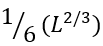 is the average number of loops protruding from the interface of
  residues. The multiplier
 ![]() results from the fact that the chain can have, roughly, 6 directions in each interface residue (4 along the interface, 1 inside the folded part, and only 1 looking outside, thereby initiating a loop). Among many possible cross-section interfaces dividing the globule into two halves, the lowest-free-energy interface should serve for the transition state on the folding/unfolding pathway. Therefore, this "optimal" interface should be covered by no more than
results from the fact that the chain can have, roughly, 6 directions in each interface residue (4 along the interface, 1 inside the folded part, and only 1 looking outside, thereby initiating a loop). Among many possible cross-section interfaces dividing the globule into two halves, the lowest-free-energy interface should serve for the transition state on the folding/unfolding pathway. Therefore, this "optimal" interface should be covered by no more than ![]() , but possibly smaller, number of loops.
, but possibly smaller, number of loops.
The value ![]() is the average number of residues in a closed loop in the transition state ( L/2 being the number of unfolded residues in the folding nucleus, and
is the average number of residues in a closed loop in the transition state ( L/2 being the number of unfolded residues in the folding nucleus, and  the number of loops there). The value
 ![]() is the entropy lost by a
is the entropy lost by a 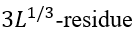 closed loop at the interface (such a loop cannot cross the interface plane; this restriction changes 3/2, the conventional Flory's coefficient for the entropy of an unrestricted closed loop, to 5/2 [Finkelstein & Badretdinov, 1997a, b]). Having L ~ 100 (actually, this approximation is good for the whole range of L = 10 - 1000), one obtains
 (3a)
(3a)
In the mid-transition ambient conditions, the transition state free energy  equals to
 ![]() . The
. The  value is not less than ΔE# - 0 (when ΔS#=0) and not larger than ΔE# - Tmelt(DS#)lower, that is,
![]() (4)
(4)
Thus, when the free energy difference ∆F between the native (most stable) and unfolded state is equal to zero, the time of both folding and unfolding of the L-residue protein chain is estimated as
![]() (5)
(5)
where τ ≈ 10 ns is the time of structure growth by one residue [Zana, 1975] (this τ is the second and the last empirical parameter used in the theory [Finkelstein & Badretdinov, 1997a, b]).
Here, one thing should be added: A search over folds with different chain knottings can, in principle, be a rate-limiting “quasi-Levinthal” factor, since the knotting cannot be changed without globule decay. However, since the computer experiments show that one chain knot involves many tens of residues, the search for correct knotting can only be rate-limiting for extremely long (L>>1000) chains [Finkelstein & Badretdinov, 1998] that cannot fold within a reasonable time (according to eq. (5)) in any case.
The above equation shows that in the mid-transition conditions (where ∆F=0), a 100-residue protein chain should attain its most stable fold within milliseconds or days, but not years.
If the native fold is more stable than the unfolded state (i.e., if ∆F<0), the folding is faster. Because the folding nucleus covers about half of the chain (more detailed calculations [Garbuzynskiy et al., 2013] give ≈40%), its free energy decreases from ![]() (that was at ∆F=0) to approximately
(that was at ∆F=0) to approximately ![]() + 0.4∆F at ∆F<0, so that
+ 0.4∆F at ∆F<0, so that
![]() (6)
(6)
which can be approximately presented as
![]() (6a)
(6a)
[Garbuzynskiy et al., 2013]. Because the value ∆F ≈ 40 kJ/mol for a ~100-residue protein under physiological conditions [Privalov, 1979], the folding time of such a protein decreases about 100-fold, and now ranges from a fraction of millisecond to a few hours.
It should be noted that all the above considerations are focused on the case of the moderate stability of the native fold, which corresponds to the available data on protein folding (occurring near the mid-transition point, see Fig. 2). For the opposite case of a very high native fold stability ![]() , another but similar to eq. (5) scaling law
, another but similar to eq. (5) scaling law ![]() was obtained by Thirumalai [1995].
was obtained by Thirumalai [1995].
Concluding: one can see that although the protein folding problem is the so-called “NP-hard” problem [Ngo & Marks, 1992; Unger, & Moult, 1993] (which loosely speaking implies an exponentially-long time to be spent to solve it by a folding chain or by a computer), and indeed the time is a stretched-exponential function of the chain length L (see eqs. (5), (6a), and the later rigorous mathematical papers [Fu & Wang, 2004; Steinhofel et al., 2006]), this does not mean that this time is unreasonably long for a normal protein domain.
7. Protein folding times: theory and experiment
The observed protein folding times (see Fig. 6) span over 11 orders of magnitude (which is akin to the difference between the life span of a mosquito and the age of the universe).
Figure 6 shows the region theoretically allowed for the folding times by equations (5) - (6a) (and obtained with only two empirical and no adjustable parameters) and describes the observed folding times of all studied single-domain globular proteins of any size and stability of their native state.
Figure 6 also shows that a chain of L≲80-90 residues will find its most stable fold within minutes (or faster) even under "non-biological" mid-transition conditions, where folding is known [Creighton, 1978; Fersht, 1999] to be the slowest (see also Fig. 2). Thus, native structures of such relatively small proteins are under complete thermodynamic control: they are the most stable among all structures of these chains.
Native structures of larger proteins (of ≈100-400 residues) are, in addition, under a kinetic "control of complexity", in a sense that too entangled folds of their long chains cannot be achieved within days or weeks even if they are thermodynamically stable; and indeed, globular domains with greatly entangled folds of long protein chains have never been observed [Garbuzynskiy et al., 2013]: they seem to be excluded from the repertoire of existing protein structures. Besides, the native fold of at least one protein (serpin) of ≈400 residues is not the most stable but a long-living metastable fold [Tsutsui et al., 2012].
The kinetic control also explains why even larger (with L≳450) proteins should have far from spherical shape or consist (according to the “divide and rule” principle) of separately folding domains: otherwise, chains of more than 450 residues would fold too slowly. This is a kinetic "size restriction" for domains. In a sense, this effect resembles Levinthal's "kinetic control", though at another level and only for very large proteins. The above estimates (≈100 and ≈400 residues) are somewhat (by 30-50%) elevated when the native fold free energy ΔF is substantially lower than that of the unfolded chain, but essentially they remain nearly the same [Garbuzynskiy et al., 2013].
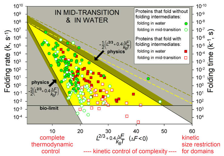
Figure 6. The folding rates and times. Experimental in vitro measurements have been made "in water" (under approximately "biological" conditions) and at mid-transition for 107 single-domain proteins (or separate domains) without SS bonds and covalently bound ligands (though the rates for proteins with and without SS bonds are principally the same [Galzitskaya et al., 2001]). The golden-and-white triangle: the region theoretically allowed by physics at the mid-transition. Its golden part corresponds to biologically-reasonable folding times (≤10 min), the bronze belt is the additional area allowed in "biological" conditions. The white zone: the larger folding times (i.e., the smaller folding rates) are observed (for some proteins) only under the mid-transition (i.e., "non-biological") conditions. The yellow dashed line limits the additional area allowed for oblate (1:2) and oblong (2:1) globules at mid-transition; the bronze dashed line means the same for “biological” conditions. L is the number of amino acid residues in the protein chain. ΔF is the free energy difference between the native and unfolded states of the chain under the experimental conditions and temperature T. Adapted from [Garbuzynskiy et al., 2013].
Equations (5) - (6a) only outline the range of folding times depending on the protein size and stability of its native structure under given ambient conditions. To predict the protein folding time more accurately, the shape of its folding nucleus or, for lack of such information, of its native fold should be taken into account; this has been done by Plaxco et al. [1998], who introduced a "contact order" (CO, that equals to the average chain separation of the residues that are in contact in the native protein fold, divided by the chain length) as a phenomenological measure of complexity of the native fold (though, only for small proteins that fold without folding intermediates). Then this CO was adjusted for the already developed [Finkelstein & Badretdinov, 1997a, b] chain length dependence, and the resulting method [Ivankov et al., 2003] has shown quite good results, now for all proteins, and the later extension of this method [Finkelstein et al., 2013] gave even more accurate results.
It should be added that no attention was paid in these works to specific structures of folding nuclei; the attention was only paid to their overall features like size, instability and complexity. The reason: there is ample evidence that in some cases, folding nuclei are well-organized and possess specific structural features (see [Fersht, 1999, 2000; Garbuzynskiy & Kondratova, 2008; Shaw et al., 2010]), while in others, they are poorly organized ("diffused nuclei") (see [Grantcharova et al., 2001; Finkelstein et al., 2007, 2014] and references therein). The latter, together with the observed sensitivity of positions and shapes of the folding nuclei to mutations, led to the conclusion that a "nucleus" is an ensemble of structures rather than a single structure, and that that the folding nucleus and folding pathway are much less resistant to amino acid sequence mutations and change of ambient conditions than the native protein structure.
Also, it should be noted that all the above considerations were focused on stability (or rather, instability) of transition states (folding nuclei) and paid virtually no attention to folding intermediates, because these - in contrast to transition states - do not determine the rate of folding of native structures [Fersht, 1999, 2000].
8. Dependence of the number of compact chain folds on the protein size
The total ("Levinthal's") volume of the protein conformation space estimated at the level of amino acid residues is huge: ≳3100 conformations for a 100-residue chain.
However, should the chain sample all these conformations in search for its most stable fold? No: a vast majority of them are non-compact (that is, high-energy ones); but the conformation space is covered by local energy minima, each surrounded by a local energy funnel (Fig. 7) providing fast downhill decent to this local minimum. And, actually, the folding protein chain has to sample only various ways of packing the chain into the compact protein globule.
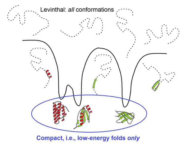
Figure 7. Comparison of a huge search among all, for the most part disordered, conformations and a much less voluminous search only among compact and well-structured globules, thus corresponding to the deep energy minima surrounded by energy funnels. Adapted from [Finkelstein, 2017].
To estimate the actual volume of this sampling, one has to estimate the number of local energy minima. This is similar to the idea of enumerating possible "topomers" that a protein chain can form [Debe et al. 1999; Makarov & Plaxco, 2003; Wallin & Chan, 2005].
An overview of protein structures shows that interactions occurring in the chains are mainly connected with secondary structures [Levitt & Chothia, 1976; Chothia & Finkelstein, 1990; Finkelstein & Ptitsyn, 2002]. Thus, a question arises as to how large the total number of energy minima is if considered at the level of formation and assembly of secondary structures into a globule, that is, at the level considered by Ptitsyn [1973] in his model of stepwise protein folding.
We will be interested mostly in proteins that fold under thermodynamic control, that is, ones having chains of L~100 or less amino acid residues (see above). Such proteins have no more than 10 α- and β-structural elements [Ptitsyn & Finkelstein, 1980; Rollins & Dill, 2014].
The number of compact globular packings of the chain is by many orders of magnitude smaller than that of conformations of amino acid residues [Finkelstein & Garbuzynskiy, 2015]: the latter, according to Levinthal’s estimate, scales up as something like 100L or 10L or 3L with the number L of residues in the chain, while the former scales up not faster (see below) than ~LN with the chain length L and the number N of the secondary structure elements. N is much less than L (N < L/10, according to Rollins & Dill [2014]), and this drastic decrease of the power N as compared to L is the main reason for the drastic decrease of the conformation space.
The number of compact globular packings of the chain with given secondary structures can be presented [Finkelstein & Garbuzynskiy, 2015] as a product of the following multipliers (Fig. 8).
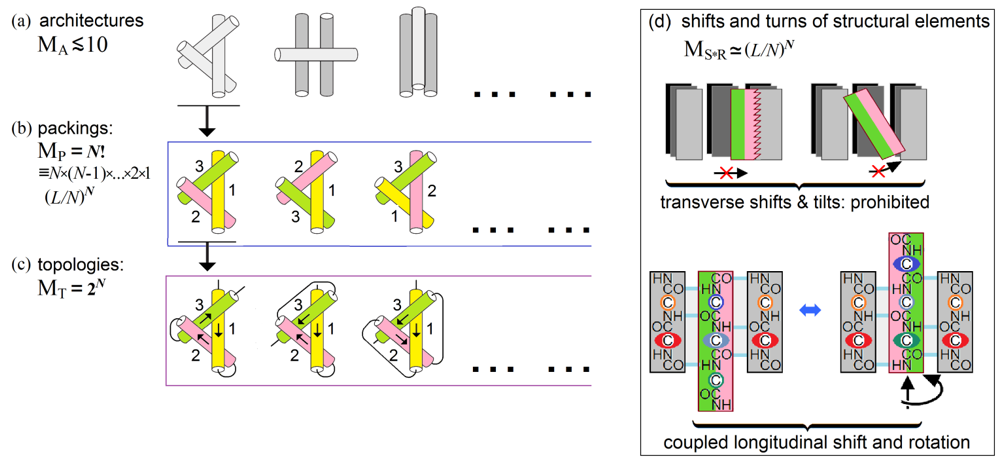
Figure 8. A scheme of estimate of the conformation space volume at the level of secondary structure assembly and packing. Explanations are given in the text. Adapted from Supplement to [Finkelstein & Garbuzynskiy, 2015].
MA, the number of architectures, i.e., types of dense stacks of given secondary structures. This number is small (cf. [Levitt & Chothia, 1976; Murzin & Finkelstein, 1988; Chothia & Finkelstein, 1990]). It is usually (at L≾100 and N≾10) ~10 or less architectures (Fig. 8a) for a given set of secondary structures, since the architectures are packings of a few secondary structure layers (each containing several secondary structures), and therefore the combinatorics of the layers is very small as compared to that of much more numerous secondary structure elements, which is described below.
MP, the number of all possible combinations of positions of N structural elements within the given protein architecture that cannot exceed ![]() .
.
MT, the number of all possible topologies, i.e., all combinations of directions of these structural elements that cannot exceed 2N (Fig. 8c).
MS*T, the number of possible shifts and turns (Fig. 8d) of structural elements within the dense globule. Here, transverse shifts and tilts are prohibited by the dense packing, while longitudinal shifts and rotations of structural elements are coupled (this is shown using a β-sheet as the best illustrative example, but this is also true for α-helices – remember “knobs in the holes” close packings by Crick [1953]); as a result, each α- or β-element can have about L/N (that is, about the element's mean length) possible shifts/turns in the globule formed by N secondary structures in the L-residue chain.
The above means that the number of compact packings of N secondary structure elements ("topomers") is ~MA•MP•MT ~ 10•N!•2N. Using Stirling's approximation (N!~(N/e)N), the number of topomers can be estimated as ~[10•(2/e)N]•NN, i.e., about NN in the main term at N>>1.
Each of these topomers contains MS*T~(L/N)N local energy minima connected with shifts and turns. As a result, the total number of energy minima in the conformational space is ![]() ~
~ ![]() conformations; this (using Stirling's approximation
conformations; this (using Stirling's approximation ![]() gives
gives
![]() (7)
(7)
in the main term (if L >> N >> 1) [Finkelstein & Garbuzynskiy, 2015].
This number can be somewhat reduced by the symmetry of the globule, by shortness of some loops, by the impossibility to have α-helices inside β-sheets, etc., but this is not important in estimating the upper limit of the number of conformations [Finkelstein & Garbuzynskiy, 2015].
As to the question of how the chain knows where and what secondary structures to form, the answer is that most of the secondary structures are determined by local amino acid sequences [Ptitsyn & Finkel'shtein, 1970; Ptitsyn, 1973; Lim, 1974a, b; Chou & Fasman, 1974; Schulz et al., 1974; Ptitsyn &Finkelstein, 1983; Finkelstein et al., 1990; Jones, 1999; etc.].
Because in a chain of L≈20 residues one (N=1) α-helix forms within ≈0.2 ms [Mukherjee et al., 2008], and a β-hairpin of N=2 β-strands forms within ≈6 ms [Muñoz et al., 1997], the time necessary for iterating ~ LN of possible assemblies of the secondary structures can be estimated (cf. eq. (6a)) as
![]() (7a)
(7a)
In a compact globule, the length of a secondary structure element should be proportional to the globule's diameter, i.e., to ~L1/3. More specifically, a diameter of a globule of L residues is ≈5L1/3Å, and thus, on the average, a helix consists of ≈3L1/3 residues, while a β-strand, as well as a loop, comprises ≈1.5L1/3 residues. Thus, (an α-glodule (consisting of α-helices connected by loops) contains ≈L/[L1/3(3+1.5)] = L2/3/4.5 helices, and a β-structural globule (consisting of β-strands connected by loops) contains of ≈L/[L1/3(1.5+1.5)] = L2/3/3 β-strands [Finkelstein & Garbuzynskiy, 2015]. This means that
NUMBER of secondary elements N ≈ L2/3/4.5 [for α-proteins] — L2/3/3 [for b-proteins]. (8)
Thus, the value LN of possible secondary structure assemblies is expected to come within the range
![]() (9)
(9)
Since ![]() , the outlined range of possible secondary structure assemblies is close to
, the outlined range of possible secondary structure assemblies is close to
![]() (9a)
(9a)
for normal domains of L~100 residues (see explanations after eq. (3)), and the number of the secondary structure assemblies scales with the chain length L approximately as the upper boundary of the range of folding times outlined by equation (6a) [Finkelstein & Badretdinov, 1997a, b].
It is not out of place mentioning that the scaling of LN given by equation (9) looks like those obtained by Fu & Wang [2004] and Steinhofel et al. [2006] from mathematical consideration of the problem complexity rather than from physical reasons.
This Entry for Encyclopedia has been written after my recent reviews [Finkelstein et al., 2017, 2018; Finkelstein, 2017, 2018; Ivankov & Finkelstein, 2020] and lectures [Finkelstein & Ptitsyn, 2016; Finkelstein, 2020].[1][2][3][4][5][6][7][8][9][10][11][12][13][14][15][16][17][18][19][20][21][22][23][24][25][26][27][28][29][30][31][32][33][34][35][36][37][38][39][40][41][42][43][44][45][46][47][48][49][50][51][52][53][54][55][56][57][58][59][60][61][62][63][64][65][66][67][68][69][70][71][72][73][74][75][76][77][78][79][80][81][82][83][84][85][86][87][88][89][90][91][92][93][94][95][96][97][98][99][100][101][102][103][104][105][106][107][108][109][110][111][112][113][114][115][116][117][118][119][120][121][122][123][124][125][126][127][128][129]
References
- Abkevich V.I., Gutin A.M., Shakhnovich E.I. 1994. Specific nucleus as a transition state for protein folding: evidence from the lattice model. Biochemistry, 33: 10026–10031.
- Anfinsen C.B. The Molecular Basis of Evolution. Chapters 5, 6. 1959. — New York: John Wiley.
- Anfinsen C.B. 1973. Principles that govern the folding of protein chains. Science, 181: 223–230.
- Anfinsen C. B., Scheraga H. A. 1975. Experimental and theoretical aspects of protein folding. Adv. Protein Chem., 29: 205–300.
- Anfinsen C.B., Haber E., Sela M., White F.H., Jr. 1961. The kinetics of formation of native ribonuclease during oxidation of the reduced polypeptide chain. Proc. Natl. Acad. Sci. USA, 47: 1309–1314.
- Bicout D.J., Szabo A. 2000. Entropic barriers, transition states, funnels, and exponential protein folding kinetics: A simple model. Protein Sci., 9: 452–465.
- Bogatyreva N.S., Finkelstein A.V. 2001. Cunning simplicity of protein folding landscapes. Protein Eng., 14: 521–523.
- Bryngelson J.D., Wolynes P.G. 1987. Spin Glasses and the Statistical Mechanics of Protein Folding. Proc. Natl. Acad. Sci. USA, 84: 7524-7528.
- Bryngelson J.D., Wolynes P.G. 1989. Intermediates and barrier crossing in a random energy model (with applications to protein folding). J. Phys. Chem., 93: 6902–6915.
- Bryngelson J.D., Onuchic J.N., Socci N.D., Wolynes P.G. 1995. Funnels, pathways, and the energy landscape of protein folding: a synthesis. Proteins, 21: 167–195.
- Chothia C., Finkelstein A.V. 1990. The classification and origins of protein folding patterns. Ann. Rew. Biochem., 59: 1007–1039.
- Chou P.Y., Fasman G.D. 1974. Prediction of protein conformation. Biochemistry, 13: 222-245.
- Creighton T.E. 1978. Experimental studies of protein folding and unfolding. Prog. Biophys. Mol. Biol., 33: 231-97.
- Crick F.H.C. 1953. The packing of -helices: Simple coiled coils. Acta Crystallogr., 6: 689–697.
- Debe D.A., Carlson M.J., Goddard W.A., 3rd. 1999. The topomer-sampling model of protein folding. Proc. Natl. Acad. Sci. USA, 96: 2596-601.
- Dill K.A., Chan H.S. 1997. From Levinthal to pathways to funnels. Nat. Struct. Biol., 4: 10–19.
- Dill K.A., MacCallum J.L. 2012. The protein-folding problem, 50 years on. Science. 338: 1042–1046.
- Djikaev Y, Ruckenstein E. 2016. Model for the nucleation mechanism of protein folding. In: Ruckenstein, E; Berim, G. 2016. Kinetic Theory of Nucleation, pp. 231-250. CRC Press, Taylor & Francis Group: Boca Raton.
- Dolgikh D.A., Kolomiets A.P., Bolotina, I.A. Ptitsyn O.B. 1984. “Molten globule” state accumulates in carbonic anhydrase folding. FEBS Lett., 164: 88–92.
- Eichmann C., Preissler S., Riek R., Deuerling E. 2010. Cotranslational structure acquisition of nascent polypeptides monitored by NMR spectroscopy. Proc .Natl. Acad. Sci. USA, 107: 9111–9116.
- Eisenberg D.S. 2018. How hard it is seeing what is in front of your eyes. Cell, 174: 8-11.
- Ellis R.J., Hartl F.U. 1999. Principles of protein folding in the cellular environment. Curr. Opin. Struct. Biol. 9: 102–110.
- Emanuel N.M., Knorre D.G. The Course in Chemical Kinetics, 4th edn. (in Russian). Chapters III (§ 2), V (§§ 2, 5). 1984.— Moscow: Vysshaja Shkola.
- Eyring H, 1935. The activated complex in chemical reactions. J. Chem. Phys., 3: 107–115.
- Fersht A.R. Structure and mechanism in protein science: A guide to enzyme catalysis and protein folding. Chapters 2, 15, 18, 19. 1999. — NY: W. H. Freeman & Co.
- Fersht A.R. 2000. Transition-state structure as a unifying basis in protein-folding mechanisms: Contact order, chain topology, stability, and the extended nucleus mechanism. Proc. Natl. Acad. Sci., 97: 1525–1529.
- Finkelstein A.V. 2002. Cunning simplicity of a hierarchical folding. J. Biomol. Struct. Dyn., 20: 311–313.
- Finkelstein A.V. 2015. Time to overcome the high, long and bumpy free-energy barrier in a multi-stage process: The generalized steady-state approach. J. Phys. Chem. B, 119: 158-163.
- Finkelstein A.V. 2017. Some additional remarks to the solution of the protein folding puzzle: Reply to comments on “There and back again: Two views on the protein folding puzzle”. Phys. Life Rev., 21: 77-79.
- Finkelstein A.V. 2018. 50+ years of protein folding. Biochemistry (Moscow), 83: S3-S18.
- Finkelstein A.V. 2020. Sounded course of lectures "Protein Physics" (in Russian) at the Lomonosov Moscow State University. https://yadi.sk/d/hBOaPER4bNX4mw.
- Finkelstein A.V., Badretdinov A.Ya. 1997a. Physical reason for fast folding of the stable spatial structure of proteins: A solution of the Levinthal paradox. Mol. Biol. (Moscow, Eng. Trans.), 31: 391-398.
- Finkelstein A.V., Badretdinov A.Ya. 1997b. Rate of protein folding near the point of thermodynamic equilibrium between the coil and the most stable chain fold. Fold. Des., 2: 115–121.
- Finkelstein A.V., Badretdinov A.Ya. 1998. Influence of chain knotting on the rate of folding. ADDENDUM to Rate of protein folding near the point of thermodynamic equilibrium between the coil and the most stable chain fold. Fold. Des., 3: 67–68.
- Finkelstein A.V., Garbuzynskiy S.O. 2015. Reduction of the search space for the folding of proteins at the level of formation and assembly of secondary structures: A new view on solution of Levinthal’s paradox. ChemPhysChem, 16: 3373-3378.
- Finkelstein A.V., Garbuzynskiy S.O. 2016. Solution of Levinthal’s paradox is possible at the level of the formation and assembly of protein secondary structures. Biophysics, 61: 1-5.
- Finkelstein A.V., Ptitsyn O.B. Protein Physics. A Course of Lectures. Chapters 7, 10, 13-21. 2002. — Amsterdam – Boston – London – New York – Oxford – Paris – San Diego – San Francisco – Singapore – Sydney – Tokyo: Academic Press, An Imprint of Elsevier Science.
- Finkelstein A.V., Ptitsyn O.B. Protein Physics.2-nd edn. 2016. — Amsterdam – Boston – Heidelberg – London – New York – Oxford – Paris – San Diego – San Francisco – Singapore – Sydney – Tokyo: Academic Press, An Imprint of Elsevier Science.
- Finkelstein A.V., Badretdinov A.Ya., Gutin A.M. 1995. Why do protein architectures have a Boltzmann-like statistics? Proteins, 23: 142-150.
- Finkelstein A.V., Badretdinov A.Yu, Ptitsyn O.B. 1990. Short alpha-helix stability. Nature, 345: 300-300.
- Finkelstein A.V., Bogatyreva N.S., Garbuzynskiy S.O. 2013. Restrictions to protein folding determined by the protein size. FEBS Letters, 587: 1884-1890.
- Finkelstein A.V., Ivankov D.N., Garbuzynskiy S.O., Galzitskaya O.V. 2007. Understanding the folding rates and folding nuclei of globular proteins. Current Protein and Peptide Science, 8: 521-536.
- Finkelstein A.V., Ivankov D.N., Garbuzynskiy S.O., Galzitskaya O.V. 2014. Understanding the folding rates and folding nuclei of globular proteins. In eBook Series "Frontiers in Protein and Peptide Sciences" (B.M. Dunn, ed.), V.1, chapter 5, pp.91-138.
- Finkelstein A.V., Badretdin A.J., Galzitskaya O.V., Ivankov D.N., Bogatyreva N.S., Garbuzynskiy S.O. 2017. There and back again: Two views on the protein folding puzzle. Phys. Life Rev., 21: 56-71.
- Finkelstein A.V., Badretdin A.J., Galzitskaya O.V., Ivankov D.N., Bogatyreva N.S., Garbuzynskiy S.O. 2018. Two views on the protein folding puzzle. In "Trends in Biomathematics: Modeling, Optimization and Computational Problems (R.P. Mondiani, ed.), pp. 391-412. Bazel: Springer Nature Switzerland AG.
- Flanagan J.M., Kataoka M., Shortle D., Engelman D.M. 1992. Truncated staphylococcal nuclease is compact but disordered. Proc. Natl. Acad. Sci. USA, 89: 748-752.
- Flory P.J. Statistical Mechanics of Chain Molecules, Chapter 3. 1969. — NY: Interscience Publishers.
- Fu B., Wang W. 2004. A 2^0(n^(1-1/d)∙log(n)) time algorithm for d-dimensional protein folding in the HP-model. Lecture Notes in Computer Science, 3142: 630–644.
- Fulton K.F., Main E.R.G., Dagett V., Jackson S.E. 1999. Mapping the interactions present in the transition state for unfolding/folding of FKBP12. J. Mol. Biol., 291: 445–461.
- Galzitskaya O.V., Finkelstein A.V. 1995. Folding of chains with random and edited sequences: similarities and differences. Protein Eng., 8: 883-892.
- Galzitskaya O.V., Finkelstein A.V. 1999. A theoretical search for folding/unfolding nuclei in three-dimensional protein structures. Proc. Natl. Acad. Sci. USA, 1999, 96: 11299-11304.
- Galzitskaya O.V., Ivankov D.N., Finkelstein A.V. 2001. Folding nuclei in proteins. FEBS Lett., 489: 113–118.
- Galzitskaya O.V., Garbuzynskiy, S.O., Ivankov D.N., Finkelstein A.V. 2003. Chain length is the main determinant of the folding rate for proteins with three-state folding kinetics. Proteins, 51: 162-166.
- Garbuzynskiy S.O., Kondratova M.S. 2008. Structural features of protein folding nuclei. FEBS Lett., 582:768-772.
- Garbuzynskiy S.O., Ivankov D.N., Bogatyreva N.S., Finkelstein A.V. 2013. Golden triangle for folding rates of globular proteins. Proc. Natl. Acad. Sci. USA, 110: 147–150.
- Go N., Abe H. 1981. Noninteracting local-structure model of folding and unfolding transition in globular proteins. I. Formulation. Biopolymers, 20: 991–1011.
- Goldenberg D.P., Creighton T.E. 1983. Circular and circularly permuted forms of bovine pancreatic trypsin inhibitor. J. Mol. Biol., 165: 407–413.
- Grantcharova V.P., Riddle D.S., Santiago J.V., Baker D. 1998. Important role of hydrogen bonds in the structurally polarized transition state for folding of the src SH3 domain. Nat. Struct. Biol., 5: 714–720.
- Grantcharova V., Alm E., Baker D., Horwich A.L. 2001. Mechanism of protein folding. Curr. Opin. Struct. Biol., 11: 70–82.
- Gutin A.M., Shakhnovich E.I. 1993. Ground state of random copolymers and the discrete random energy model. J. Chem. Phys., 98: 8174–8177.
- Han Y., David A., Liu B., Magadan J.G., Bennink J.R., Yewdell J.W., Qian S.B. 2012. Monitoring cotranslational protein folding in mammalian cells at codon resolution. Proc. Natl. Acad. Sci. USA, 109: 12467–12472.
- Holtkamp W., Kokic G., Jäger M., Mittelstaet J., Komar A.A., Rodnina M.V. 2015. Cotranslational protein folding on the ribosome monitored in real time. Science, 350: 1104-1107.
- Ivankov D.N., Finkelstein A.V. - Solution of the Levinthal's paradox and a physical theory of protein folding times. – Biomolecules, 2020, 10(2), E250; doi: 10.3390/biom10020250.
- Ivankov D.N., Garbuzynskiy S.O., Alm E., Plaxco K.W., Baker D., Finkelstein A.V. 2003. Contact order revisited: Influence of protein size on the folding rate. Protein Sci., 12: 2057–2062.
- Isenman D.E., Lancet D., Pecht I. 1979. Folding pathways of immunoglobulin domains. The folding kinetics of the C3 domain of human IgG1. Biochemistry, 18: 3327-3336.
- Jackson S.E. 1998. How do small single-domain proteins fold? Fold. Des., 3:R81–R91.
- Jacobson H., Stockmayer W. 1950. Intramolecular reaction in polycondensations. I. The theory of linear systems. J. Chem. Phys., 18: 1600-1606.
- Jones D.T. 1999. Protein secondary structure prediction based on position-specific scoring matrices. J. Mol. Biol., 292: 195–202; current version of the program: http://bioinf.cs.ucl.ac.uk/psipred/.
- Karplus M. 1997. The Levinthal paradox: yesterday and today. Fold. Des., 2, Suppl. 1: S69–S75.
- Kolb V.A., Makeev E.V., Spirin A.S. 1994. Folding of firefly luciferase during translation in a cell-free system. EMBO J., 13: 3631–3637.
- Komar AA, Kommer A, Krasheninnikov IA, Spirin AS. Cotranslational folding of globin. 1997. J. Biol. Chem., 272: 10646–10651.
- Landau L.D., Lifshitz E.M. Statistical Physics. (Volume 5 of A Course of Theoretical Physics). 3-rd edn. §§ 7, 8, 150. 1980. — Amsterdam – Boston – Heidelberg – London – New York – Oxford – Paris – San Diego – San Francisco – Singapore – Sydney – Tokyo: Elsevier.
- Lappalainen I., Hurley M.G., Clarke J. 2008. Plasticity within the obligatory folding nucleus of an immunoglobulin-like domain. J. Mol. Biol., 375: 547–559.
- Leopold P.E., Montal M., Onuchic J.N. 1992. Protein folding funnels: a kinetic approach to the sequence-structure relationship. Proc. Natl. Acad. Sci. USA, 89: 8721–8725.
- Levinthal C. 1968. Are there pathways for protein folding? J. Chim. Phys. Chim. Biol., 65: 44–45.
- Levinthal C. 1969. How to fold graciously. In: Mössbauer Spectroscopy in Biological Systems: Proceedings of a meeting held at Allerton House, Monticello, Illinois (P. Debrunner, J.C.M. Tsibris, E. Munck, eds.). — University of Illinois Press: Urbana-Champaign, IL, pp. 22–24.
- Levitt M., Chothia C. 1976. Structural patterns in globular proteins. Nature, 261: 552–558.
- Libich D.S., Tugarinov V., Clore G.M. 2015. Intrinsic unfoldase/foldase activity of the chaperonin GroEL directly demonstrated using multinuclear relaxation-based NMR. Proc. Natl. Acad. Sci. USA, 112: 8817–8823.
- Lim V.I., 1974a. Structural principles of the globular organization of protein chains. A stereochemical theory of globular protein secondary structure. J. Mol. Biol. 88: 857–872.
- Lim V.I., 1974b. Algorithm for prediction of _-helices and _-structural regions in globular proteins. J. Mol. Biol. 88: 873–894.
- Makarov D.E., Plaxco K.W. 2003. The topomer search model: A simple, quantitative theory of two-state protein folding kinetics. Protein Sci., 12: 17-26.
- Marchenko N.Y., Garbuzynskiy S.O., Semisotnov G.V. 2009. Molecular chaperones under normal and pathological conditions. In "Molecular Pathology of Proteins" (D.I. Zabolotny, ed.), pp. 57–89. New York: Nova Science Publishers.
- Marchenko N.Y., Marchenkov V.V., Semisotnov G.V., Finkelstein A.V. 2015. Strict experimental evidence that apo-chaperonin GroEL does not accelerate protein folding, although it does accelerate one of its steps. Proc. Natl. Acad. Sci. USA, 112: E6831–6832.
- Marchenkov V.V., Sokolovskiĭ I.V., Kotova N.V., Galzitskaya O.V., Bochkareva E.S., Girshovich A.S., Semisotnov G.V. 2004. The interaction of the GroEL chaperone with early kinetic intermediates of renaturing proteins inhibits the formation of their native structure. Biofizika (in Russian), 49: 987–994.
- Matouschek A., Kellis J.T., Serrano L., Fersht A.R. 1990. Transient folding intermediates characterized by protein engineering. Nature. 346: 440–445.
- Mukherjee S., Chowdhury P., Bunagan M. R., Gai F. 2008. Folding kinetics of a naturally occurring helical peptide: implication of the folding speed limit of helical proteins. J. Phys. Chem. B, 112: 9146-9150.
- Muñoz V., Thompson P.A., Hofrichter J., Eaton W.A. 1997. Folding dynamics and mechanism of beta-hairpin formation. Nature, 390: 196-199.
- Murzin A.G., Finkelstein A.V. 1988. General architecture of -helical globule. J. Mol. Biol., 204: 749-770.
- Ngo J.T., Marks J. 1992. Computational complexity of a problem in molecular structure prediction. Protein Eng., 5: 313–321.
- Nölting B. Protein Folding Kinetics: Biophysical Methods. Chapters 10, 11, 12. 2010. — NY: Springer.
- Neira J.L., Fersht A.R. 1999a. Exploring the folding funnel of a polypeptide chain by biophysical studies on protein fragments. J.. Mol.. Biol., 285: 1309–1333.
- Neira J.L., Fersht A.R. 1999b. Acquisition of native-like interactions in C-terminal fragments of barnase. J. Mol. Biol., 287: 421–432.
- Petsko G.A., Ringe, D. 2004. Protein Structure and Function. Chapter 1. London: New Science Press.
- Phillips D.C. 1966. The three-dimensional structure of an enzyme molecule. Sci. Am. 215: 78–90.
- Plaxco K.W., Simons K.T., Baker D. 1998. Contact order, transition state placement and the refolding rates of single domain proteins. J. Mol. Biol., 277: 985–994.
- Pauling L. General chemistry. Chapter 16. 1970. — NY: W.H. Freeman & Co.
- Privalov P.L. 1979. Stability of proteins: small globular proteins. Adv. Protein Chem., 33: 167–241.
- Ptitsyn O.B. 1995. Molten globule and protein folding. Adv. Protein Chem. 47: 83–229.
- Ptitsyn O.B. 1973. Stages in the mechanism of self-organization of protein molecules. Dokl. Akad. Nauk SSSR (in Russian), 210: 1213-1215.
- Ptitsyn O.B., Finkel'shtein A.V. 1970. Relation of the secondary structure of globular proteins to their primary structure. Biofizika (in Russian), 15(5): 757-768.
- Ptitsyn O.B., Finkelstein A.V. 1980. Similarities of protein topologies: evolutionary divergence, functional convergence or principles of folding? Quart. Rev. Biophys., 13: 339–386.
- Ptitsyn O.B., Finkelstein A.V. 1983. Theory of protein secondary structure and algorithm of its prediction. Biopolymers, 22: 15-25.
- Robson B, Vaithilingam A. 2008. Protein folding revisited. Prog. Mol. Biol. Transl. Sci., 84: 161–202.
- Rollins G.C., Dill K.A. 2014. General mechanism of two-state protein folding kinetics. J. Am. Chem. Soc., 136: 11420-11427.
- Ruckenstein, E; Berim, G. 2016. Kinetic Theory of Nucleation, pp. 231-250. CRC Press, Taylor & Francis Group: Boca Raton.
- Šali A., Shakhnovich E., Karplus M. 1994. Kinetics of protein folding. A lattice model study of the requirements for folding to the native state. J. Mol. Biol., 235: 1614–1636.
- Segava S., Sugihara M. 1984. Characterization of the transition state of lysozyme unfolding. I. Effect of protein-solvent interactions on the transition state. Biochemistry, 23: 2473–2488.
- Senior A.W., Evans R., Jumper J., Kirkpatrick J., Sifre L., Green T., Qin C., Žídek A., Nelson A.W.R., Bridgland A., Penedones H., Petersen S., Simonyan K., Crossan S., Kohli P., Jones D.T., Silver D., Kavukcuoglu K., Hassabis D. 2019. Protein structure prediction using multiple deep neural networks in the 13th Critical Assessment of Protein Structure Prediction (CASP13). Proteins, 87: 1141–1148.
- Senior A.W., Evans R., Jumper J., Kirkpatrick J., Sifre L., Green T., Qin C., Žídek A., Nelson A.W.R., Bridgland A., Penedones H., Petersen S., Simonyan K., Crossan S., Kohli P., Jones D.T., Silver D., Kavukcuoglu K., Hassabis D. 2019. Improved protein structure prediction using potentials from deep learning. Nature, 577: 706–710.
- Schulz G.E., Barry C.D., Friedman J., Chou P.Y., Fasman G.D., Finkelstein A.V., Lim V.I., Ptitsyn O.B., Kabat E.A., Wu T.T., Levitt M., Robson B., Nagano K. 1974. Comparison of predicted and experimentally determined secondary structure of adenyl kinase. Nature, 250: 140-142.
- Shakhnovich E.I., Finkelstein A.V. 1989. Theory of cooperative transitions in protein molecules. I. Why denaturation of globular protein is the first order phase transition. Biopolymers, 28: 1667-1680.
- Shakhnovich E.I., Gutin A.M. 1990. Implications of thermodynamics of protein folding for evolution of primary sequences. Nature, 346: 773–775.
- Shakhnovich E.I. 2006. Protein folding thermodynamics and dynamics: where physics, chemistry, and biology meet. Chem. Rev. 106: 1559-1588.
- Shaw D.E., Maragakis P., Lindorff-Larsen K., Piana S., Dror R.O., Eastwood M.P., Bank J.A., Jumper J.M., Salmon J.K., Shah Y., Wriggers W. 2010. Atom-level characterization of structural dynamics of proteins. Science, 330, 341–346.
- Steinhofel K., Skaliotis A., Albrecht A.A. 2006. Landscape analysis for protein folding simulation in the H-P model. Lecture Notes in Computer Science, 4175: 252–261.
- Thirumalai D. 1995. From minimal models to real proteins: time scales for protein folding kinetics. J. Phys. I. (Orsay, Fr.), 5: 1457–1469.
- Tanford C. 1968. Protein denaturation. Adv. Protein Chem., 23: 121–282.
- Tsutsui Y., Cruz R.D., Wintrode P.L. 2012. Folding mechanism of the metastable serpin α1-antitrypsin. Proc. Natl. Acad. Sci. USA, 109: 4467–4472.
- Unger R., Moult J. 1993. Finding the lowest free energy conformation of a protein is an NP-hard problem: proof and implications. Bull. Math. Biol., 55: 1183–1198.
- Wallin S., Chan H.S. 2005. A critical assessment of the topomer search model of protein folding using a continuum explicit-chain model with extensive conformational sampling. Protein Sci., 14: 1643–1660.
- Wang J., Oliveira R.J., Chu X., Whitford P.C., Chahine J., Han W., Wang E., Onuchic J.N., Leite V.B. 2012. Topography of funneled landscapes determines the thermodynamics and kinetics of protein folding. Proc. Natl. Acad. Sci. USA, 109: 15763–15768.
- Wensley B.G., Gärtner M., Choo W.X., Batey S., Clarke J. 2009. Different members of a simple three-helix bundle protein family have very different folding rate constants and fold by different mechanisms. J. Mol. Biol. 390: 1074–1085.
- Wetlaufer D.B. 1973. Nucleation, rapid folding, and globular intrachain regions in proteins. Proc. Natl. Acad. Sci. USA, 70: 697–701.
- Wolynes P.G. 1997. Folding funnels and energy landscapes of larger proteins within the capillarity approximation. Proc. Natl. Acad. Sci. USA, 94: 6170–6175.
- Wolynes P.G. 2015. Evolution, energy landscapes and the paradoxes of protein folding. Biochimie, 119: 218–230.
- Wolynes P.G., Onuchic J.N., Thirumalai D. 1995. Navigating the folding routes. Science, 267: 1619–1620.
- Yang J., Anishchenko I., Park H., Peng Z., Ovchinnikov S., Baker D. 2020. Improved protein structure prediction using predicted interresidue orientations. Proc. Natl. Acad. Sci. USA, 117: 1496-1503.
- Zana R. 1975. On the rate determining step for helix propagation in the helix-coil transition of polypeptides in solution. Biopolymers, 14: 2425–2428.
- Zwanzig R., Szabo A., Bagchi B. 1992. Levinthal's paradox. Proc. Natl. Acad. Sci. USA, 89: 20–22.