Your browser does not fully support modern features. Please upgrade for a smoother experience.
Submitted Successfully!
 +1 credit
Thank you for your contribution! You can also upload a video entry or images related to this topic.
For video creation, please contact our Academic Video Service.
| Version | Summary | Created by | Modification | Content Size | Created at | Operation |
|---|---|---|---|---|---|---|
| 1 | Umed Singh Panu | -- | 4524 | 2024-03-06 19:16:10 | | | |
| 2 | Rita Xu | Meta information modification | 4524 | 2024-03-07 03:41:52 | | |
Video Upload Options
We provide professional Academic Video Service to translate complex research into visually appealing presentations. Would you like to try it?
Cite
If you have any further questions, please contact Encyclopedia Editorial Office.
Sharma, T.C.; Panu, U.S. Hydrological Droughts. Encyclopedia. Available online: https://encyclopedia.pub/entry/55936 (accessed on 24 July 2026).
Sharma TC, Panu US. Hydrological Droughts. Encyclopedia. Available at: https://encyclopedia.pub/entry/55936. Accessed July 24, 2026.
Sharma, Tribeni C., Umed S. Panu. "Hydrological Droughts" Encyclopedia, https://encyclopedia.pub/entry/55936 (accessed July 24, 2026).
Sharma, T.C., & Panu, U.S. (2024, March 06). Hydrological Droughts. In Encyclopedia. https://encyclopedia.pub/entry/55936
Sharma, Tribeni C. and Umed S. Panu. "Hydrological Droughts." Encyclopedia. Web. 06 March, 2024.
Copy Citation
Hydrological droughts may be referred to as sustained and regionally extensive water shortages as reflected in streamflows that are noticeable and gauged worldwide. The analysis of hydrological droughts is largely conducted using the truncation level approach to represent the desired demand level of water equivalent to the median, mean, or any other flow quantile of an annual, monthly, or weekly flow sequence.
copula
extreme number theorem
entropy
Markov chains
1. Introduction to Hydrological Droughts
Several definitions have been proposed for hydrological droughts. Yevjevich [1] defined the hydrological drought as a period with water content below the average water content in streams, reservoirs, aquifers, lakes, and soils. This period is associated with the effects of precipitation shortfall on surface and subsurface water supply, rather than with direct shortfalls in precipitation. In recent years, Tallaksen and van Lanen [2] defined the hydrological drought as a sustained and regionally extensive occurrence of below-average water availability. Hydrological droughts can cover extensive areas and can last for months to years, with devastating impacts on the ecological system and many economic sectors such as drinking water supply, crop production (irrigation), waterborne transportation, electricity production (hydropower or cooling water), and recreational activities (rowing, boating, etc., due to low water levels in lakes, rivers, reservoirs, etc.). The other deleterious impact of the hydrologic drought is the deterioration of the water quality as a consequence of the decline in water quantity in the surface water bodies. Almost all studies on hydrologic droughts have used streamflows as the drought variable primarily due to the wide availability of recorded streamflow time series across the globe. It is for this reason that while dealing with droughts based on streamflows, the term streamflow drought is also commonly used.
1.1. Time Scales of Hydrological Droughts
The hydrological drought analysis began with the annual scale (annual droughts) as pioneered by Yevjevich [1] and associates [3][4]. This work on an annual scale was extended by Dracup et al. [5], Sen [6], Guven [7], Yevjevich [8], Lee et al. [9], Horn [10], Fernandez and Salas [11], Sharma [12], Salas et al. [13], Panu and Sharma [14], Akyuz et al. [15], Sen [16], among others. The yearly analysis offered theoretical simplification as the annual flow sequences can be perceived as stationary in the statistical and stochastic sense. The stationarity requirement eased the application of the existing theories of probability and stochastic processes, which paved the way for further analysis on a short time basis such as month and week. Although the annual scale is rather long, it can be used to abstract information on the regional behavior of hydrologic droughts and the assessment of equivalent deficit volumes that need to be stored in the reservoirs on a long-term basis. An appropriate time scale for the analysis of hydrological droughts can be deemed as a month [17][18][19][20][21][22][23][24][25][26][27][28][29] because of the consideration that a month is a reasonable time unit for monitoring drought effects in situations related to water supply, groundwater abstraction, crop irrigation, management of reservoirs for hydropower generation, etc. However, it is to be noted that Wu et al. [27] used multiple time scales (month to year) using non-standardized streamflow indices. Also, for the hydrologic design of reservoirs in the context of dams, a monthly scale of flows is considered adequate [17][25], and thus, the drought magnitude-based analysis with a monthly scale is very apt. In recent years, Sharma and Panu [24][30], and Gurrapu et al. [31] have extended the analysis to a weekly scale for assessing duration and associated water shortages within a year or a season, while reckoning the strong persistence characteristics of hydrologic droughts on a short time basis. It is well known that the operational drought forecasts are traditionally issued on a weekly basis such as Palmer drought severity indices and Palmer moisture anomaly indices, which make weekly analysis very desirable. Further, weekly analysis is a more precise way of assessing the water needs during drought periods on an emergency and crisis basis. Additionally, weekly analysis provides a complementary way of testing the validity of drought models developed on a monthly scale, as the periodic or non-stationary effects on flow sequences are imbued on both time scales [24]. For studying the behavior of short-term droughts within a year or a season, the daily scale has also been used [2][23][32][33][34][35][36][37][38][39][40][41].
1.2. Parameters of Hydrological Droughts
Hydrological drought is characterized by a multitude of parameters but chiefly by (a) duration; (b) magnitude (earlier called severity); (c) time of initiation and cessation; and (d) areal spread. At times, the term magnitude is complemented by the intensity, which is defined as magnitude/duration by Dracup et al. [5]. Conceptually, the above drought parameters can be illustrated in terms of an untransformed (or historical) flow sequence (Figure 1A) and a transformed (or standardized) flow sequence (Figure 1B).
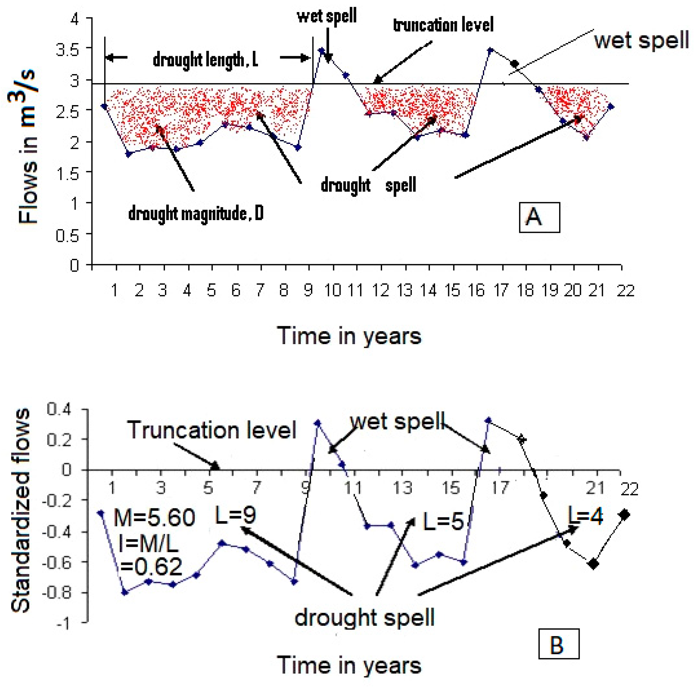
Figure 1. Definition sketch of hydrological drought parameters: (A) natural (or untransformed) flow sequence and (B) standardized (or transformed) flow sequence.
Natural (or untransformed) form means a sequence of annual flows {xi (m3/s)} as they are observed and recorded in the field, and later on reported in the hydrological yearbooks or related websites, whereas the standardized form means {xi} is transformed to {ei} such that {ei = (xi − μ)/σ}, where μ and σ are mean and standard deviation of xi sequence, and thus, {ei} sequence has mean = 0 and standard deviation = 1.
It should be mentioned that in the earlier literature from the 1960s until recently (say the early part of the first decade of the 21st century, i.e., 2000–2006) on hydrologic droughts, the term severity was used to denote the cumulative deficit. The cumulative deficit is named as magnitude in the context of meteorological droughts or when the drought variable is precipitation [42][43][44]. The usage of the term magnitude in contrast to the term severity is increasing over time [19][24][45]. This transition seems to be motivated by ambiguity in the meaning of the term “severity”. In the context of meteorological drought, severity is expressed to indicate the rigor or the category of the drought such as mild, moderate, severe, or extreme. For example, Palmer [46] suggested an index that now is popularly known as the “Palmer drought severity index “(PDSI)” to indicate the severity of drought from mild (PDSI < −1.0) to extreme (PDSI < −4). Likewise, another index termed the standardized precipitation index (SPI) suggested by Mckee et al. [42][43] is being currently used to denote the category (mild, moderate, severe, extreme) of the severity of meteorological droughts. In the context of hydrological droughts, the severity denotes a deficit in volumetric or depth units, and therefore, its usage contradicts the index connotation associated with meteorological droughts. The term magnitude alleviates this anomaly and is also in sync with the volume (essentially magnitude) connotation associated with the cumulative deficit.
The most basic element for deriving the above parameters is the truncation level which divides the time series (or sequence) of the desired drought variable such as streamflow into sections named as “deficit” and “surplus”. The parameters of a drought such as duration, magnitude, and intensity are the properties of the deficit sections. Consequently, the duration (L) has the unit of time such as year, month, week, or day, depending on the time unit of variable manifesting the drought. For instance, when dealing with monthly streamflows, drought duration will be registered/recorded in months. The term deficit (D) refers to the cumulative shortage (sum of individual deficit epochs in a drought episode) below the chosen demand level (or the so-called truncation level), and it has the unit of volume, i.e., m3. It should be borne in mind that the truncation level in the parlance of hydrologic drought is representative of the demand level of water to be met by a river in the equivalent form. For example, in a river, if the water needs are assessed as equivalent to the mean flow of the river; then, the truncation level can be taken as the long-term mean flow. In reservoir design, the demand level is taken preferably as 75% of the mean annual flow (also known as a draft) [25][47]; so, under such a situation, the truncation level may correspond close to the median (Q50, i.e., flows exceeding or equal to 50% of the time in a flow duration curve). In most cases, the median (Q50) is considered to be a better choice as the mean annual flow imposes a significantly high value of draft, resulting in exceptionally large size of reservoirs. The drought duration and deficit can be analyzed in the standardized form for the ease of interpretation and the possible inter-comparison of drought scenarios in varied environments. For a standardized flow sequence, the deficit is termed as magnitude and denoted by M (=D/σ; Yevjevich [1]), which is a dimensionless quantity. However, the unit of duration (L) remains unchanged and consequently would have a time unit of month or year depending on whether a monthly or annual flow sequence is being analyzed as the drought variable. Therefore, a value of L = 9 (Figure 1) in the standardized domain is tantamount to L = 9 years for the case when the analysis is carried out on a yearly sequence of the drought variable. The quantity M/L is termed as the drought intensity (I). The longest run length for a sample size of T years (or equivalently of the return period of T-year) is denoted as LT and the corresponding deficit as DT (or MT in the standardized form of the sequence of a drought variable). Similar connotations apply when the analysis is being carried out on a monthly or weekly basis, i.e., T would represent the return period in months or weeks. In mathematical terms, MT = I × LT; DT = σ × MT, with T being the time in year(s), month(s), or week(s) of the streamflow sequences considered for analysis. The term deficit (D) is tantamount to reservoir volume.
1.3. A Note on the Choice of Truncation Level for Identification of Hydrological Droughts
Yevjevich [1] introduced the concept of the truncation level approach and statistical theory of runs in the analysis and modeling of hydrologic droughts. The truncation level specifies some statistics of the drought variable, which may be a constant or a function of time. Several investigators have considered it as a long-term mean or a median flow [1][5][6][7][12][14]. At times, it can be construed as a very relaxed criterion, simply because droughts are unlikely to be tangible at such a level of truncation. In general, a drought is perceived when the flows in a river are low, rocks in the riverbed may protrude in the air, lake and groundwater levels are low, and wells tend to run dry. It is for this reason that truncation levels such as Q70 (flows exceeding or equal to 70% of the time in a flow duration curve), Q90, Q95, etc., are used for identifying the droughts in flow series. It is because of this consideration that recent researchers [23][32][33][38] have preferred other percentile levels from the flow duration curve ranging from Q50 to Q95. In a statistical sense, the truncation level at the mean flow simplifies the analysis on a seasonal (monthly) scale, meaning that the drought is considered to occur when the flow drops below the mean of the respective month. Likewise, when one takes the median (Q50) or Q70 as the truncation level, the flow is deemed to drop below the Q50 or Q70 flow of the respective month. These threshold values of flow are not uniform even though the probability of occurrence of drought is uniform throughout 12 months. When the analysis is conducted in terms of the standardized streamflows (named SSI), the truncation level becomes uniform and equal to zero only for the situation in which the truncation level is the mean. At other flow levels, the truncation level will feature as a curve with respect to time, yet the probability of drought would remain the same for all months. Thus, the non-uniform flow cut-offs can easily absorb the climate change and/or land use changes for the hydrologic drought analysis. The same argument applies to the impact of truncation levels on the reservoir storage requirements. Specifically, at high drafts (high truncation levels), the storage requirements would increase, whereas at low drafts, the storage needs would be minimized with a greater risk of the reservoir running dry. This is the reason that an optimal truncation level for reservoir analysis is taken as 75% of the mean annual flow [25][47]. Further, the truncation level and the corresponding drought probability will be governed by the pdf of monthly flow sequences, and the linkage relationships are documented by Sharma [12]. On an annual basis, the truncation level on plotting will be a straight line, and the corresponding drought probability will be dictated by the pdf of the annual flow sequence [12]. The truncation level (Q50, Q70, etc.), in terms of changed flows in the wake of climate change or land use considerations in a catchment, can be moved up or down appropriately.
A flow duration curve could be constructed based on annual, monthly, weekly, or daily flow sequences. For the near-normal probability distribution function (pdf) of streamflow, the mean serves the purpose of a truncation level, whereas, for skewed distributions, the median should be used as a better measure of truncation level [24]. For the design and planning of a water storage system on a permanent or a long-term basis for ameliorating drought events, the use of a truncation level corresponding to the mean or median level of flow, for example, would result in a conservative design alluding to the need for a desirable drought mitigation scenario. In a regional drought frequency analysis, on the contrary, a value of the truncation level such as Q70 or Q80 would portray more tangible drought impacts over the region. However, in a short-term contingency planning for drought amelioration where drought impacts are vividly tangible, one could conduct drought investigations even at Q90 to allow for the mobilization of resources on a cost-effective basis. In the design of reservoirs, the draft is normally taken as 75% of the mean annual flow [47]; therefore, the truncation level of 75% of the mean annual flow is a wise consideration [25]. Irrespective of the truncation level, some anomalies persist in the process of delineating the dry (or drought) and wet periods. For example, if two drought spells, each of five months are separated by a wet spell, say of one month, then a natural question arises whether this one month has eliminated the drought or the drought is still persisting even during this (wet) month. It is obvious that although the flows during this month are above the cut-off level, it does not state that drought impacts on the river ecology, fish habitat, and other environmental and water use concerns are over during such a short period of a month. Likewise, when two long wet spells are broken by a dry spell of one or two months, then the dry spell is unlikely to be perceived as a drought. Under such a situation, the effects of wet spells are still rampant. The concerns arising from the above issues on the hydrological drought identification were recognized by Zelenhasic and Salvai [32], which led them to improvise the identification procedure as follows. They used Q90 or Q95 as the truncation level and observed that when the flow exceeds the threshold level for a short period of time, a long drought tends to be segmented into several small droughts, which were also found to be mutually dependent. Such an observation led to the consideration of some pooling procedures where small drought events could be pooled together to define an independent sequence. Therefore, they devised a method named inter-event-time and volume-criterion (IC) for pooling together small drought events. Also, two other methods, i.e., a moving average procedure (MA) and a sequent peak algorithm (SPA), have been suggested by Tallaksen et al. [33] for resolving the above problem while using truncation levels such as Q50, Q70, and Q90. Further, a comparative analysis of the aforesaid three methods, i.e., IC, MA, and SPA, led [33] to the inference that IC and MA methods were comparable, whereas the SPA method tended to be restrictive in terms of drought durations and less satisfactory at higher truncation levels. The inter-event-time of 5 days (IC method, meaning that any contiguous drought events separated by an inter-event-time of 5 days or less) were pooled together, and the averaging period of 11 days (MA method) was found satisfactory for two Danish catchments [33]. Tate and Freeman [36] found that the IC method was satisfactory for Zimbabwean rivers with an inter-event time of 6 days. On daily flows, Fleig et al. [38] tested the above three methods on 16 rivers across the globe and found the MA procedure to be the most flexible and worthy of recommendation.
1.4. Indices of Hydrological Droughts
The indices in the realm of hydrological droughts are still in the phase of development, and none can be said to be widely acceptable unlike the Palmer drought severity index (PDSI) [46] and standardized precipitation index (SPI) [22][42][43][44][48][49] in the arena of meteorological droughts. Since hydrological droughts are more related to the declining levels of surface water resources and primarily to streamflow, the interest has been more on the quantification of drought magnitudes for assessing shortages of water supplies during the extended periods of droughts. The truncation level approach advanced by Yevjevich [1] has therefore been rigorously applied for quantifying drought magnitudes of varying return periods. Consequently, the efforts have focused on developing conservative estimates of drought magnitudes based on the long-term mean or median as the truncation level of streamflow time series, even though droughts at this truncation level may not be tangible in the river basin, and hence, lower truncation levels may be more desirable such as Q70. For water supply situations, an index named as surface water supply index (SWSI) was developed as a measure of surface water status for the state of Colorado by Shafer and Dezman [50] to complement the PDSI by integrating snowpack, reservoir storage, streamflow, and precipitation at high elevations. Since SWSI has a scale similar to PDSI, both SWSI and PDSI are used together to trigger the drought assessment and response plan for the state of Colorado. The SWSI has been modified and adopted by other western states in the USA (Oregon, Montana, Idaho, and Utah) and is computed primarily for river basins [51][52] situated in these states. Another prominent index that falls under the purview of hydrological droughts is the PHDI (Palmer hydrological drought index) [53].
Recently, some attempts have been made to develop the indices for hydrological droughts in tandem with meteorological droughts such as SRI (standardized runoff index) [54], SDI (streamflow drought index) [55][56], and SHI (standardized hydrological index) [24][25][57]. Indices such as SDI and SRI are essentially standardized and normalized to characterize the hydrological droughts with respective time units (i.e., annual or monthly scales). It should be borne in mind that SRI and SDI are derived from the lognormal pdf of the monthly flow sequences. Nalbantis and Tsakiris [55] have defined four states for the hydrological droughts, i.e., mild drought (−1 ≤ SDI < 0); moderate drought (−1.5 ≤ SDI < −1.0); severe drought (−2 ≤ SDI < −1.5); and extreme drought (SDI < −2.0), in sync with drought states defined by SPI for meteorological droughts.
In the context of hydrological droughts, the standardized streamflow is named a standardized hydrological index (SHI) by Sharma and Panu [24][25], which is not a normalized index but follows a gamma pdf. It should be noted that SPI is standardized and normalized, whereas SHI is only standardized but not normalized. On monthly and weekly scales, the standardization implies the month-by-month or week-by-week standardization in the aforesaid indices. WMO [49] has used the term standardized streamflow index (SSI), which can be regarded as a general term with offshoots such as SRI, SDI, and SHI. Zalokar and Kobold [28] have used the term SSI, which is a term synonymous to SHI used by Sharma and Panu [24]. The SSI has been derived (normalized) for several pdfs of streamflow sequences other than gamma and lognormal [21]. Since SSI is an analogous term to SPI, therefore, it seems to have gained better acceptance in the parlance of the hydrologic drought [20][26][58][59]. A review highlighting the merits and shortcomings of various indices concerning meteorological, hydrological, and agricultural droughts is provided by Mishra and Singh [60].
2. Hydrological Drought Modeling—Relevant Preliminaries
2.1. Identification of the Probability Distribution of Streamflow Sequence as a Drought Variable
The modeling of droughts (or more aptly the drought parameters) begins with the identification of the underlying probability distribution (i.e., pdf) of the streamflow sequence, where streamflow acts as the drought variable. For identifying the underlying pdf of the drought variable, the product moment and L-moment (the linear combination of product moments) are the most popular tools. The mathematical aspects of L-moments are described well by Hosking and Wallis [61]. In the product moment method, the plot between skewness (γ) and coefficient of variation (cv) provides a clue on the probable underlying pdf. For a normal pdf, the γ is 0 irrespective of cv. To reaffirm the hypothesis of the underlying normality of a sequence of size N, the standard statistical test [0 ± 1.96 × (6/N)0.5] corresponding to a 95% confidence level for a normal distribution, vis à vis sample values of γ can be used. In the case of a gamma pdf, the scatter of points corresponding to the sampling estimates of γ and cv should lie around a straight line defined by γ = 2cv. Likewise, for a lognormal pdf, the points related to the estimated γ and cv should scatter around the theoretical curve defined by γ = 3cv + cv3. In the ambit of the L-moments, the plots of L-skewness and L-kurtosis, respectively, are designated as τ-3 and τ-4, which tend to be better descriptors of the pdf of data. There are characteristic plots of the L-skewness and L-kurtosis for pdfs such as normal, gamma, lognormal, etc., which can be matched with the sampling estimates of these parameters. The product moment and L-moment diagrams are complementary to each other in the process of identifying pdf. It should be noted that the stable estimates of L-moments require a large sample size, which is generally available for monthly, weekly, or daily time series of a drought variable. On the other hand, an annual sequence, commonly, has a small sample size, typically (N < 100), such that a good amount of useful information is unlikely to result from the L-moment analysis. In such a case, the product moment method can be regarded as sufficient, or other methods of identification such as a plot on a normal probability paper or significance test on γ = 0 should be considered.
2.2. Identification of Dependence Structure in the Streamflow Sequence
The dependence structure of the data can be ascertained by computing autocorrelations at lags 1, 2, 3, ---,10. For a Markov process, the autocorrelations at increasing lags tend to decay exponentially. The tests for the significance of autocorrelations at various lags are well described by Box et al. [62], which can be used to infer the order of dependence (random, Markov order-1 or Markov order-2, etc.). To validate the hypothesis of independence or randomness of a sequence (size N), the standard statistical tests [0 ± 1.96 × (1/N)0.5 corresponding to 95% confidence limits for randomness vis à vis sample values of autocorrelations] can be employed. In addition, Box et al. [62] have suggested the use of a chi-square statistic (called as Portmanteau statistic) based on the initial (16 to 25) values of the autocorrelations to infer independence in the sequence.
2.3. A Note on the Theory of Runs as Used in Drought Modeling
The theory of runs is well developed in the ambit of statistics and probability, which can be transposed for analyzing the drought phenomenon [4][8]. The segments (or sequels) of wet (surplus) or drought (deficit) values as shown in part-A, and part-B (Figure 1) can be regarded as runs. The wet values can be designated as “w”, whereas drought values as “d”. Therefore, the flow sequence shown in part-A or part-B (Figure 1) can be written as dddddddddwwdddddwwdddd. This sequence comprises five runs of which three runs represent drought spells and two runs represent wet spells. It is obvious and also stated for clarity that each drought event or episode is tantamount to a run. The length of a run is equivalent to the drought duration and a run sum is equivalent to the drought magnitude. The first run has a length of nine, implying the drought duration is of 9 years. The area under the red dots is the run sum. When the analysis is conducted in the standardized domain, the sequence of d’s and w’s of the drought variable remains the same with the length of the first run as nine (i.e., drought duration of 9 years) and the run sum (i.e., standardized drought magnitude, M of 5.60, with no units attached). On the yearly scale, 9 means 9 years, and hence, M = 5.60 × (σ × 365 × 24 × 60 × 60) m3 (i.e., σ in m3/s is converted into m3/year). When one is dealing with monthly streamflows, then the drought duration is 9 months, and the standardized drought magnitude M = 5.60 × (σ × 30 × 24 × 60 × 60) m3. The sequential occurrences of d’s could be random or may follow some dependence structure (the simplest being the Markov dependence). In simple terms, the number of runs (or the number of drought events) can be modelled using the Poisson probability law, the length of run (i.e., the drought duration) can be modelled using geometric probability law, and likewise, the drought intensity (= magnitude/duration) can be modelled by the truncated normal pdf. Thus, the theory of runs provides a powerful tool for the analysis of parameters of hydrological droughts.
One major requirement for the application of the theory of runs is that the time series of a drought variable must be at least weakly stationary in the statistical sense. The requirement of stationarity is generally met for the annual precipitation (or streamflow) sequence of the drought variable. The sequence of monthly or weekly streamflows is non-stationary and must be transformed into a stationary time series. The month-by-month or week-by-week standardization renders the non-stationary series into a stationary one which can readily be subjected to hydrological drought analysis by the theory of runs. Once a suitable probability distribution fitting a monthly or weekly flow sequence is ascertained, the underlying dependence structure of such a flow sequence can be investigated as briefly described below.
For a flow sequence {xy,t} comprising of the tth month (t = 1, 2, 3,……,12) in the yth year (1 ≤ y ≤ N), the standardized series {uy,t = (xy,t − μt)/σt} with μt and σt, respectively, being the mean and standard deviation of the tth month is rendered as a stationary sequence with mean zero and variance one. Since {uy,t} series is non-periodic and stationary stochastic, it can be designated as {ei, 1 ≤ i ≤ n (=12 × N}. In the case of a weekly sequence, “t” ranges from 1 to 52, and n = 52 × N. Hence, there are 52 μ’s and 52 σ’s for the weekly flows, whereas 12 sets of μ’s and σ’s stand for the monthly flows. It is recognized that {ei} is a standardized series but not a normalized one because its generic source {xy,t} is generally non-normal for a monthly or a weekly flow sequence. For an annual sequence, {ei} can be obtained by standardizing an annual sequence {xi} by a set of μ and σ (i.e., ei = (xi − μ)/σ, 1 ≤ i ≤ N). The {ei} series being stationary (with mean 0 and standard deviation 1) can be analyzed using the theory of runs. Since {ei} series is standardized, it is referred to as the Standardized Hydrologic Index (SHI) series in the ensuing text. When SHI is normalized, it is called SSI, developed by WMO and GWP [49].
References
- Yevjevich, V. An Objective Approach to Definitions and Investigations of Continental Hydrologic Drought; Hydrology Paper 23; Colorado State University: Fort Collins, CO, USA, 1967.
- Tallaksen, L.; van Lanen, H. Hydrological drought. In Processes and Estimation Methods for Streamflow and Groundwater; Elsevier: Amsterdam, The Netherlands, 2004.
- Millan, J.; Yevjevich, V. Probabilities of Observed Droughts; Hydrology Paper 50; Colorado State University: Fort Collins, CO, USA, 1971.
- Salazar, P.G.; Yevjevich, V. Analysis of Drought Characteristics by the Theory of Runs; Hydrology Paper 80; Colorado State University: Fort Collins, CO, USA, 1975.
- Dracup, J.A.; Lee, K.S.; Paulson, E.G., Jr. On identification of droughts. Water Resour. Res. 1980, 16, 289–296.
- Sen, Z. Statistical analysis of hydrological critical droughts. J. Hydraul. Eng. 1980, 106, 99–115.
- Guven, O. A simplified semi-empirical approach to the probability of extreme hydrological droughts. Water Resour. Res. 1983, 19, 441–453.
- Yevjevich, V. Methods for determining statistical properties of droughts. In Coping with Droughts; Yevjevich, V., da Cunha, L., Vlachos, E., Eds.; Water Resources Publications: Littleton, CO, USA, 1983; pp. 22–43.
- Lee, K.S.; Sadeghipour, J.; Dracup, J.A. An approach for frequency analysis of multiyear drought durations. Water Resour. Res. 1986, 22, 655–662.
- Horn, D.R. Characteristics and spatial variability of droughts in Idaho. J. Irrig. Drain. Eng. 1989, 115, 111–124.
- Fernandez, B.; Sales, J.D. Return period and risk of hydrologic events. II. applications. J. Hydrol. Eng. 1999, 4, 308–316.
- Sharma, T.C. Drought parameters in relation to truncation level. Hydrol. Proc. 2000, 14, 1279–1288.
- Salas, J.; Fu, C.; Cancelliere, A.; Dustin, D.; Bode, D.; Pineda, A.; Vincent, E. Characterizing the severity and risk of droughts of the Poudre River, Colorado. J. Water Resour. Plan. Manag. 2005, 131, 383–393.
- Panu, U.S.; Sharma, T.C. Analysis of annual hydrologic droughts: A case of the northwest Ontario, Canada. Hydrol. Sci. J. 2009, 54, 29–42.
- Akyuz, D.E.; Bayazit, M.; Onoz, B. Markov chain models for hydrological drought characteristics. J. Hydrometeorl. 2012, 13, 298–309.
- Sen, Z. Applied Drought Modelling, Prediction and Mitigation; Elsevier Inc.: Amsterdam, The Netherlands, 2015.
- Burn, D.H.; Wychreschul, J.; Bonin, D.V. An integrated approach to the estimation of streamflow drought quantiles. Hydrol. Sci. J. 2004, 49, 1011–1024.
- Shiau, J.T.; Feng, S.; Nadarajah, S. Assessment of hydrological droughts for the Yellow River China using copulas. Hydrol. Proc. 2007, 21, 2157–2163.
- Lopez-Moreno, J.I.; Vicente-Serrano, S.M.; Beguria, S.; Garcia-Ruiz, J.M.; Portela, M.M.; Almeida, A.B. Dam effects on drought magnitude and duration in a transboundary basin: The lower River Tagus, Spain and Portugal. Water Resour. Res. 2009, 45, W02405.
- Lorenzo-Lacruz, J.; Vicente-Serrano, S.M.; Gonzalez-Hidalgo, J.C.; Lopez-Moreno, J.I.; Cortesi, N. Hydrological drought response to meteorological drought in the Iberian Peninsula. Clim. Res. 2013, 58, 117–131.
- Vicente-Serrano, S.M.; Lopez-Moreno, J.I.; Beguria, S.; Lorenzo-Lacruz, J.; AzorinMolin, C.; Moran-Tejeda, E. Accurate computation of streamflow drought index. J. Hydrol. Eng. 2012, 17, 318–322.
- Vicente-Serrano, S.M.; Dominguez-Castro, D.C.; McVicar, T.R.; Thomas-Burguera, M.; Pena-Gallardo, M.; Noguera, M.; Lopez-Moreno, J.I.; Pena, D.; Kenaway, A.E. Global characterization of hydrological and meteorological droughts under future climate change: The importance of time scale, vegetation-CO2 feedbacks and change to distribution functions. Int. J. Clim. 2020, 40, 2557–2567.
- Sung, J.H.; Chung, E.-S. Development of streamflow drought severity-duration-frequency curves using the threshold level method. Hydrol. Earth Syst. Sci. 2014, 18, 3341–3351.
- Sharma, T.C.; Panu, U.S. Modeling of hydrological droughts: Experiences on Canadian streamflows. J. Hydrol. Reg. Stud. 2014, 1, 92–106.
- Sharma, T.C.; Panu, U.S. A drought magnitude-based method for reservoir sizing: A case of annual and monthly flows from Canadian rivers. J. Hydrol. Reg. Stud. 2021, 36, 100829.
- Rad, A.M.; Ghahraman, B.; Khalili, D.; Ghabremani, Z.; Ardakani, S.A. Integrated meteorological and hydrological drought model: A management tool for proactive water resources planning in semi-arid regions. Adv. Water Resour. 2017, 107, 336–353.
- Wu, J.; Chen, X.; Love, C.A.; Yao, H.; Chen, X.; AghaKouchak, A. Determination of water required to recover from hydrological drought: Perspective for drought propagation and non-standardized indices. J. Hydrol. 2020, 590, 125227.
- Zalokar, L.; Kobold, M. Investigation on spatial and temporal variability of hydrological droughts in Slovenia using SSI. Water 2021, 13, 3197.
- Botai, C.M.; Botai, J.O.; dewit, J.P.; Ncongwane, K.P.; Murambadoro, M.; Barasa, P.M.; Adelo, A.M. Hydrological drought assessment based on the standardized streamflow index: A case study of the three cape provinces of South Africa. Water 2021, 13, 3498.
- Sharma, T.C.; Panu, U.S. A procedure for estimating drought duration and magnitude at a uniform cutoff of streamflow: A case of weekly flows from Canadian rivers. Hydrology 2022, 9, 109.
- Gurrapu, S.; Sauchyan, D.J.; Hodder, K.R. Assessment of hydrological drought risk in Calgary, Canada using weekly river flows of the past millennium. J. Water Clim. Chang. 2022, 13, 1920–1935.
- Zelenhasic, E.; Salvai, A. A method of streamflow drought analysis. Water Resour. Res. 1987, 23, 156–168.
- Tallaksen, L.M.; Madsen, S.; Clausen, B. On definition and modelling of streamflow deficits and volume. Hydrol. Sci. J. 1997, 42, 15–33.
- Kjeldsen, T.R.; Lundroff, A.; Rosbjberg, D. Use of two-component exponential distribution in partial duration modelling of hydrological droughts in Zimbabwean rivers. Hydrol. Sci. J. 2000, 45, 285–298.
- Tate, E.I.; Freeman, S.N. Three modelling approaches for seasonal streamflow droughts in southern Africa: The use of censored data. Hydrol. Sci. J. 2000, 45, 27–42.
- Demuth, S.; Stahl, K. (Eds.) ARIDE-Assessment of the Regional Impact of Droughts in Europe; A Final Report; Institute of Hydrology, University of Freiburg: Freiburg im Breisgau, Germany, 2001.
- Zaidman, M.D.; Rees, H.G.; Young, A.R. Spatio-temporal development of streamflow droughts in northwestern Europe. Hydrol. Earth Syst. Sci. 2002, 6, 733–751.
- Fleig, A.K.; Tallaksen, L.M.; Hisdal, H.; Demuth, S. A global evaluation of streamflow drought characteristics. Hydrol. Earth Syst. Sci. 2006, 10, 532–552.
- Fleig, A.K.; Tallaksen, L.M.; Hisdal, H.; Hannah, D.M. Regional hydrological drought in north-western Europe: Linking a new regional drought area index with the weather type. Hydrol. Proc. 2011, 25, 1163–1179.
- van Huijgevoort, M.H.J.; Hazenburg, P.; van Lanen, H.A.J.; Uijlenhoet, R. A generic method for hydrological drought identification across different climate regions. Hydrol. Earth Syst. Sci. 2012, 16, 2437–2451.
- van Loon, A.F.; Laaha, G. Hydrological drought severity explained by climate and catchment characteristics. J. Hydrol. 2015, 26, 3–14.
- McKee, T.B.; Doesen, N.J.; Kleist, J. The relationship of drought frequency and duration to time scales. In Proceedings of the 8th Conference on Applied Climatology, Anaheim, CA, USA, 17–22 January 1993; pp. 179–184.
- McKee, T.B.; Doesen, N.J.; Kleist, J. Drought monitoring with multiple time scales. In Proceedings of the 9th conference on Applied Climatology, Dallas, TX, USA, 15–20 January 1995; pp. 233–236.
- Heim, H.M., Jr. A review of twentieth-century drought indices used in the United States. Bul. Am. Meteorol. Soc. 2002, 83, 1149–1165.
- Timilsena, J.; Piechota, T.C.; Hidalgo, H.; Tootle, G. Five hundred years of hydrological drought in the upper Colorado River basin. J. Am. Water Resour. Asso. 2007, 43, 798–812.
- Palmer, W.C. Meteorological Droughts; Paper No. 45; Weather Bureau, U.S. Dept. of Commerce: Washington, DC, USA, 1965; pp. 1–58.
- McMahon, T.A.; Adeloye, A.J. Water Resources Yield; Water Resources Publications: Littleton, CO, USA, 2005.
- Guttman, N.B. Accepting the standardized precipitation index: A calculation algorithm. J. Am. Water Resour. Asso. 1999, 30, 311–322.
- World Meteorological Organization (WMO); Global Water Partnership (GWP). Handbook of Drought Indicators and Indices (M. Svoboda and B.A. Fuchs); Integrated Drought Management Programme (IDMP), Integrated Drought Management Tools and Guidelines Series 2: Geneva, Switzerland, 2016.
- Shafer, B.A.; Dezman, E.A. Development of a surface water supply index (SWSI) to assess the severity of drought conditions in the snowpack runoff area. In Proceedings of the 50th Annual Western Snow Conference; Colorado State University: Fort Collins, CO, USA, 1982; pp. 164–175.
- Dosken, N.J.; Garen, D. Drought monitoring in the western United States using a surface water supply index. In Proceedings of the Seventh Conference on Applied Climatology, Salt Lake City, UT, USA, 10–13 September 1991; American Meteorological Society: Boston, MA, USA, 1991; pp. 266–269.
- Garen, D.C. Revised surface water supply index for the western United States. J. Water Resour. Plan. Manag. 1993, 119, 437–454.
- Keyantash, J.; Dracup, J.A. The quantification of drought: An evaluation of indices. Bul. Am. Meteorol. Soc. 2002, 83, 1167–1180.
- Shukla, S.; Wood, A.F. Use of standardized runoff index for characterizing hydrologic drought. Geophys. Res. Let. 2008, 35, L02405.
- Nalbantis, I.; Tsakris, G. Assessment of hydrological drought revisited. Water Resour. Manag. 2009, 23, 881–897.
- Tabari, H.; Nikbakht, J.; Talaee, P.H. Hydrological drought assessment in northeastern Iran based on streamflow drought index (SDI). Water Resour. Manag. 2013, 27, 137–151.
- Yeh, C.F.; Wang, J.; Yeh, H.F.; Lee, C.H. SDI and Markov chain for regional drought characteristics. Sustainability 2015, 7, 10789–10808.
- Tijdeman, E.; Stahl, K.; Tallaksen, L.M. Drought characteristics derived based on the standardized streamflow index: Large sample comparison for parametric and non-parametric methods. Water Resour. Res. 2020, 5610, 20119WR026315.
- Teutschbein, C.; Montano, B.Q.; Todorovic, A.; Grabs, T. Streamflow droughts in Sweden: Spatiotemporal patterns emerging from six decades of observations. J. Hydrol. Reg. Stud. 2022, 42, 101171.
- Mishra, A.K.; Singh, V.P. A review of drought concepts. J. Hydrol. 2010, 391, 202–216.
- Hosking, J.R.M.; Wallis, J.R. Regional Frequency Analysis: An Approach Based on L-Moments; Cambridge University Press: Cambridge, UK, 1997.
- Box, G.E.P.; Jenkins, G.M.; Reinsel, G.C.; Ljung, G.M. Time Series Analysis, Forecasting and Control, 5th ed.; Wiley: Hoboken, NJ, USA, 2015.
More
Information
Subjects:
Engineering, Civil
Contributors
MDPI registered users' name will be linked to their SciProfiles pages. To register with us, please refer to https://encyclopedia.pub/register
:
View Times:
1.1K
Revisions:
2 times
(View History)
Update Date:
07 Mar 2024
Table of Contents


Notice
You are not a member of the advisory board for this topic. If you want to update advisory board member profile, please contact office@encyclopedia.pub.
OK
Confirm
Only members of the Encyclopedia advisory board for this topic are allowed to note entries. Would you like to become an advisory board member of the Encyclopedia?
Yes
No
${ textCharacter }/${ maxCharacter }
Submit
Cancel
Back
Comments
${ item }
|
${ item.createdUser.fullName }
${ item.createdAt }
${ item.vote }
${ item.reply }
Delete
${ reply.createdUser.fullName }
${ reply.createdAt }
${ reply.vote }
Delete
There is no reply to this comment~
${ item.replyTextCharacter }/${ item.replyMaxCharacter }
Submit
Cancel
More
No more~
There is no comment~
${ textCharacter }/${ maxCharacter }
Submit
Cancel
${ selectedItem.replyTextCharacter }/${ selectedItem.replyMaxCharacter }
Submit
Cancel
Confirm
Are you sure to Delete?
Yes
No