Your browser does not fully support modern features. Please upgrade for a smoother experience.
Submitted Successfully!
 +1 credit
Thank you for your contribution! You can also upload a video entry or images related to this topic.
For video creation, please contact our Academic Video Service.
| Version | Summary | Created by | Modification | Content Size | Created at | Operation |
|---|---|---|---|---|---|---|
| 1 | Hamed Etezadi | -- | 7895 | 2024-02-21 06:04:45 |
Video Upload Options
We provide professional Academic Video Service to translate complex research into visually appealing presentations. Would you like to try it?
Cite
If you have any further questions, please contact Encyclopedia Editorial Office.
Etezadi, H.; Eshkabilov, S. Control Algorithms of Agriculture Autonomous All-Terrain Vehicles. Encyclopedia. Available online: https://encyclopedia.pub/entry/55261 (accessed on 27 July 2026).
Etezadi H, Eshkabilov S. Control Algorithms of Agriculture Autonomous All-Terrain Vehicles. Encyclopedia. Available at: https://encyclopedia.pub/entry/55261. Accessed July 27, 2026.
Etezadi, Hamed, Sulaymon Eshkabilov. "Control Algorithms of Agriculture Autonomous All-Terrain Vehicles" Encyclopedia, https://encyclopedia.pub/entry/55261 (accessed July 27, 2026).
Etezadi, H., & Eshkabilov, S. (2024, February 21). Control Algorithms of Agriculture Autonomous All-Terrain Vehicles. In Encyclopedia. https://encyclopedia.pub/entry/55261
Etezadi, Hamed and Sulaymon Eshkabilov. "Control Algorithms of Agriculture Autonomous All-Terrain Vehicles." Encyclopedia. Web. 21 February, 2024.
Copy Citation
This review paper discusses the development trends of agricultural autonomous all-terrain vehicles (AATVs) from four cornerstones, such as (1) control strategy and algorithms, (2) sensors, (3) data communication tools and systems, and (4) controllers and actuators, based on 221 papers published in peer-reviewed journals for 1960–2023. The paper highlights a comparative analysis of commonly employed control methods and algorithms by highlighting their advantages and disadvantages. It gives comparative analyses of sensors, data communication tools, actuators, and hardware-embedded controllers. In recent years, many novel developments in AATVs have been made due to advancements in wireless and remote communication, high-speed data processors, sensors, computer vision, and broader applications of AI tools. Technical advancements in fully autonomous control of AATVs remain limited, requiring research into accurate estimation of terrain mechanics, identifying uncertainties, and making fast and accurate decisions, as well as utilizing wireless communication and edge cloud computing. Furthermore, most of the developments are at the research level and have many practical limitations due to terrain and weather conditions.
all-terrain vehicles
control algorithm
sensor
actuator
autonomous vehicles
agricultural ATVs
1. Introduction
Autonomous all-terrain vehicle (AATV)-based farming promises to produce more crops with less effort and reduce environmental impact. Drones, self-driving all-terrain vehicles, and seed-planting robots could play a crucial role in future food supplies. According to the Global Market Insights report, the autonomous farm equipment market is projected to grow at over 6% CAGR between 2021 and 2027. By 2027, industry shipments are expected to exceed 210,000 units. Growth in the market is likely to be augmented by the growing demand for autonomous farming equipment, especially in regions with a low farmer population. Autonomous farm equipment market growth has been negatively impacted by the COVID-19 pandemic. Several governments have imposed travel restrictions and lockdown measures in response to the outbreak. As a result, several companies’ logistics and manufacturing capabilities have been hindered, resulting in lower sales figures. Additionally, the introduction of travel regulations increased labor shortage challenges for farm owners and restricted their ability to hire suitable workers to conduct fieldwork [1]. Food chains are being affected by global farming shortages. With reference to the agriculture and agri-food labor task force [2], there may be 114,000 labor shortages in Canada’s farming sector by 2025. The situation is similar in the US, where immigration changes have contributed to a shortage of farm labor. The use of AATVs can improve management by facilitating in-field tasks in a time-effective manner. A rise in farm labor costs and a fall in self-driving technology prices will also accelerate the transition. A growing body of evidence suggests that precision agriculture is already saving growers money and increasing yields. A 10% increase in farmer revenue could be achieved, as well as a reduction in labor costs [3]. In addition to their lighter weight, the AATVs would reduce soil compaction because of their compact size, which can reduce crop yields and has been a problem with heavy tractor machinery in the past.
AATVs, which are mostly four-wheel vehicles and are now used for a variety of purposes [4], are primarily used in agricultural fields for moving, carrying tools, applying chemical fertilizers, plowing, mowing grass, spreading seeds, transporting livestock, weed detection [5], and transporting firewood.
In agricultural operations, farmers are faced with different fields, each of which has its own characteristics depending on the type of product or desired operation, and these machines must perform as correctly as possible in these fields. In this regard, for future intelligent manned and/or unmanned agricultural operations, a review of the management of agricultural machinery was presented. Strategic, tactical, operational, and evaluation aspects of mechanization [6]. Among this machinery, ATVs play an essential role in agricultural operations. The special features of ATVs, such as low-pressure tires, short axle distances, narrow track widths, and high centers of gravity, make them maneuverable [7].
Considering the numerous uses and versatility of ATVs, they form a dynamic field of study. It is crystal clear that terrain properties influence the design, performance, and mobility of vehicles. Better traction and minimal sinkage will increase maneuverability, especially in wet terrain. In other words, a significant objective is to reduce the amount of roll, reduce steering effort, and thus enhance stability. As a result of increased maneuverability, vehicles have to be more stable on the road, especially in rough terrain. It is possible to reduce 85% of fatal events in agriculture by improving the balance control of these tools [8]. Any system failure in an ATV may lead to irreversible consequences [9]. Detecting such faults accurately and timely is crucial to preventing critical hazards and halting operations. For this reason, supervisory intelligent control algorithms and controllers should be continuously monitored in a smart setting to maximize ATV uptime and prevent potential hazards [10]. Therefore, the importance of control systems in ATVs is crucial.
There are a few crucial issues to be considered while designing and building autonomous ATVs that need to be investigated and improved, such as safety, especially against overturning, being autonomous, using the latest artificial intelligence technologies, and high-precision navigation. Improvement in each of these cases will increase the output and farmers’ work efficiency. Experimental studies have been conducted on maintaining the balance of AATVs [11]. Turning at low speed on surfaces with uneven slopes and sharp turns on flat ground were included in these tests, and the car’s condition was assessed statically and dynamically, but these tests were not repeatable because of remote control by radio control [11], and considering human errors, the need for automatic speed control and steering control systems in these kinds of experiments was deemed to be imperative [11]. An AATV was modeled, simulated, and tested on a test track [12]. The purpose of this study was to examine the degree to which simplified ADAMS modeling can accurately simulate the response of an AATV on uneven ground. The researchers concluded that chassis flexibility affects the vibration response of the vehicle body in a significant way [12].
Wireless communication. In another experiment, using wireless control, Aras modified the ATV to have semi-autonomous control. Yaw motion was used to determine the ATV’s stability. The ATV model was inferred using the MATLAB system identification toolbox based on the results of the experiment or yaw motion [13]. A vehicle’s motion is greatly influenced by rolling resistance, especially when it is operating off-road. As a result of reduced rolling resistance, smaller motors can be implemented, which will reduce manufacturing costs, reduce vehicle weight, reduce energy loss, and reduce rolling resistance further. Petterson and Gooch presented new data for the rolling resistance of seven different ATV tires in an agricultural environment [14]. They found rolling resistance is heavily influenced by the diameter of ATV tires. Despite large tire diameters, significant tire width and a wide, deep tread were found to adversely affect rolling resistance. The rolling resistance increased with speed at low speeds, and inflation pressure affected rolling resistance significantly.
Rolling resistance. Rolling resistance is strongly influenced by the firmness of the ground. In contrast to hard surfaces (such as concrete), soft soils (such as sand) produce a much higher resistance force. Rolling resistance is also influenced by the ground surface. Compared with tires driven on smooth surfaces, tires driven on rough macro- or micro-textures will experience greater deformation and suffer larger energy losses [15].
Terramechanics. From the terrain mechanics aspect, there are three general categories of modeling for ATVs: (1) empirical models, the simplest models but difficult to apply beyond testing conditions; (2) physics-based models, exhibiting the greatest degree of fidelity but at the expense of a high computational expenditure; and (3) semi-empirical models, which are better suited for real-time estimation and control because they strike a balance between computational efficiency and fidelity [16]. One of the most widely used semi-empirical methods is the Bekker-based model [17,18]. For Bekker-based models to produce an accurate representation of the complex stress distribution generated at the contact patch, several parameters are considered, such as cohesion and internal friction angle. In ATV operation, however, it is difficult to determine these parameters because vehicles may operate on terrain that is unknown or whose properties vary. In addition, SCM was used, but since stress is discretized and integrated, this method may not be suitable for real-time applications due to its computational cost [19]. Other methods, such as the Bekker-based SCM surrogate model, were developed to get better results. However, model-dependent navigation algorithms, such as MPC, were difficult to use due to the lack of twice-continuous differentiability [20]. Using a neural network terramechanics model for terrain estimation, the tire’s lateral forces can be predicted with sufficient accuracy [20].
Operational environment. Agricultural AATVs, unlike other conventional autonomous vehicles, cannot be controlled using traffic signs, road lanes, or other road guidance tools for navigation on the farm. Therefore, the navigation system of AATVs is the most essential part that differs from that of on-road autonomous vehicles. Plans [21], perceptions [22], and control are major parts of an autonomous navigation system, as they make up the majority of its components. ATV researchers have also conducted research in the field of navigation, analyzing the effect of algorithms such as artificial neural networks (ANNs), genetic algorithms (GAs), and Kalman filters (KFs) to enhance the accuracy of vehicle control concerning a selected route [23]. As Mousazadeh [23] concluded, an intelligent autonomous system would be enhanced by combining all categorized algorithms. Kalman filters for precise navigation, machine vision for detecting crops and rows, neural networks for weed and plant classification, fuzzy systems for detecting obstacles, and other techniques would also be required. Moreover, the review presented by Zhou and others [24] addresses path-planning problems involving multiple constraints. According to their classification, there are three stages: stage 1—structural, kinematic, and dynamic; stage 2—planning the route; and stage 3—planning the trajectory and motion, as well as a review of various methods used for USVs [24].
Studies have also been conducted to determine the correct route for USVs in the fields of route planning and motion planning, kinematics, and dynamics to design an optimal control of such vehicles [24]. Another study used LoRa-based lidar sensors in electric ATVs to predict movement paths by using data collected by the automatic driving algorithm. Using the high-resolution LiDAR scanning system developed by Rus, an automated driving algorithm was developed to map an enclosure to be used for autonomous driving purposes. To predict the location of the autonomous vehicle, a LoRa communication system was correlated with the LiDAR-type scanning system [25].
Automated vehicles currently range from (completely manual) to (fully autonomous) [26].
A vehicle’s operation is entirely under the control of the driver. However, there is still the possibility of alerting the driver in case of a danger (fully manual).
Self-driving vehicles can be classified into six levels. The levels, which are defined by the Society of Automotive Engineers (SAE), and the process of driving a vehicle vary depending on the degree of human interaction.
L0: Fully human-operated and no assistance while driving.
L1: Driver assistance systems assist drivers while driving. As well as controlling the speed of the vehicle, the steering wheel can also be maneuvered by the system (driving assistance).
L2: Driving a vehicle is a shared responsibility between the driver and the automatic system. In addition to controlling the vehicle’s speed and turning the steering wheel, the car’s speed can also be monitored by the driver (partial automation).
L3: In an autonomous vehicle, the environment can be monitored, and the vehicle can drive itself as well. Driving is permissible, but drivers have to remain in charge if necessary (conditioned automation).
L4: This system does not require human intervention; it can drive itself, it can monitor its surroundings, and it can monitor its environment as well (high automation).
L5: In any road or environment, it can drive autonomously, without human intervention (fully autonomous).
ATVs used in agriculture have been the subject of valuable studies [28,29]. A variety of navigation sensors (machine vision, GPS, laser sensors, reckoning sensors, IMUs, and GDS) were used to develop positioning and orientation control algorithms and controllers. They have also included various computational methods as well as navigation planning algorithms for agricultural vehicles (AVs). There have been numerous research publications on the designs, control algorithms, and methods employed by sensors. However, there are limited published papers on the comparative analysis of settings and performances of the employed sensors, algorithms, and control methods, communication tools and methods, control systems, and uncertainties in the study environments of AATVs. Moreover, the published papers do not cover sufficiently in-depth technical aspects of employed platforms, operational functions, sensors, internal or external communication methods, control units, and test environments of AATVs in conjunction. Another important point is that many guidance systems and their components are commercialized [29]. Therefore, many essential technical details of the guidance systems are not available.
One of the potential advantages of automated ATVs is that they are capable of reducing human-operator errors while providing stable and acceptable results and more accurate control in the long run [11,30]. The same is true for autonomous ATVs.
ATVs with self-driving control systems have several advantages, including reducing mortality, reducing overturning, especially in rough conditions, and eliminating human error in control [11,30]. Moreover, autonomous ATVs increase the accuracy of calculations, reduce labor costs, compensate for labor shortages, and enable cameras and robotic tools with artificial intelligence to be used in precision agriculture while reducing production and operating costs, particularly in products such as sugar beets and carrots that are sensitive to compaction [31]. A study was conducted on the development of unmanned autonomous ATVs using the remote-control system method [32]. Road routing, speed control, and wheel and brake systems were tested along with three models of the autonomous command control system. Platforms equipped with sensors and actuators can be specially developed or used as hardware. As part of the robotic system, many components can be implemented on the platform, including a steering wheel that can be controlled, a computer connected to a programmable electronic control unit, as well as ports (input and output) for sensors and actuators to connect and communicate.
In agriculture, the autonomous concept will lead to the development of new equipment based on small, intelligent machines capable of performing various tasks more efficiently and environmentally friendly. Using smart tractors [33], for instance, the farmland and people can be kept safe by generating operational routes and avoiding field obstacles intelligently.
AATVs have become prominent in precision agriculture (PAG) thanks to the efficient use of information and communication technology tools to monitor crop yields and employ variable-rate technologies on farms [34]. Due to the growing agricultural knowledge system, large amounts of data are available. Based on a recent review, it was found that 37% of robotic systems are four-wheel drive, and 22.06% are used for weeding. Furthermore, 50% of the navigation systems are equipped with cameras, 20% with RTK/GNSS/INS, and 16% with LiDAR [35]. According to these statistical data, a large amount of data are used by AATVs to have an optimal result in real-time operations.
The PAG research trends could also benefit from the fifth- and sixth-generations of communication (5G and 6G). The next generation of wireless communication technologies, 5G and 6G, feature high-frequency electromagnetic waves and low latency [36]. Compared to previous wireless communication technologies, these networks offer faster data transmission speeds and greater throughput, providing device communications, user-side artificial intelligence (AI) algorithms, distributed fault diagnosis methods, and complex security strategies that may be useful in agriculture [37]. The main challenge of this technology is the lack of network infrastructure in all regions, as well as spectrum availability and implementation difficulties. There are currently security concerns, and it is an expensive technology.
From an environmental aspect, due to the complexity and dynamic nature of the work environment, challenges may arise from agricultural environments with varying conditions, canopy structures, and physio-chemical properties [38]. Each environment may have its own features and limitations. Depending on the weather conditions, such as rain, fog, or dust, the sensor function may be adversely affected. When working in an open field, lighting conditions, wind, and muddy soil may present different challenges to the sensor. Navigating in orchards can be challenging due to the surrounding trees. A major problem in paddy fields is muddy soil and the difficulty of maneuvering. Designing an ATV should take the farming environment into account [39]. Agricultural farm fields face several complicated factors. For example, working areas generally remain the same; it is easy to place landmarks around the corners of a field and consider them stationary. Generally, the plants are the same, and they can be identified easily [29].
In PAG operations, AATVs are in high demand for maneuvering and accuracy in navigation. Developing a fully autonomous ATV capable of navigating and overcoming obstacles reliably is a challenging task. To plan a vehicle’s drive path and maneuver the vehicle, it is essential to be able to correctly estimate the vehicle’s dynamic behaviors, such as stability, controllability, and maneuverability, which are directly linked with terrain conditions, such as soil properties and obstacles, in real-time. The terrain can be classified based on topography and soil mechanics parameters by integrating ground and environmental data systems. To minimize energy consumption, an energy cost-to-go map of the unstructured environments can be coupled with a model predictive controller that uses higher-fidelity models to capture important aspects of off-road energy consumption, including terra-mechanics, altitude variations, and the dynamics of the vehicle [40]. In addition, an index of wheel mobility performance can be extended to a vehicle mobility performance index, and a combination of the parameters could be used to describe the vehicle’s technical productivity and efficiency, enabling the estimation and control of vehicle mobility performance as well as facilitating the design of autonomous control systems [41].
3. Models and Control Algorithms
In an uncertain or contested environment, autonomous control systems (ACS) enable the self-governance of vehicle control functions with little to no human intervention. They are developed using model-based engineering, artificial intelligence (AI), machine learning (ML), and data acquisition. An AATV can be controlled by three elements: (1) actuators and sensors serve as a reliable base for the ATV through which digital signals are used to control the handlebars of the ATV in a forward direction; (2) speed feedback controls; and (3) brake controls. Regarding the steering control system, an AI model with an image processing system using real-time images can be used. Moreover, with the help of a trained machine learning model, it is possible to pass the current position of the ATV and the expected trajectory to the CAN bus, which is used to steer the ATV with the help of the handlebar angle expected to be built on the predicted trajectory [43]. Using different types of control strategies is another aspect of ATVs’ control systems. There are different types of control systems: PID, adaptive, open-loop controls, and closed-loop controls. PID controllers, encoders, and DC motors control the steering system of autonomous vehicles. Encoders and PID controllers are used to control systems based on the required conditions. As the steering wheel turns, the encoder generates pulses, which are sent to the DC motor attached to the front axle that turns the vehicle. Using feedback from the error value, it is possible to correct the required navigation parameters by using a PID controller. A PID controller has three built-in functions, which are proportional-integral derivative, to control the error. PID controllers are popular due to their easy-to-control and easy-to-implement capabilities.
Open-loop controls and closed-loop controls each have different situations when they are needed. In open-loop control systems, there is no feedback or error handling required. Despite its simplicity and economy, it cannot be optimized. Open-loop control systems are easier to maintain. Control systems with closed loops handle feedback and errors. In closed-loop control, feedback is the key difference. The advantages of closed-loop controls include automatic correction of disturbances, the ability to maintain a set point, and the ability to stabilize unstable processes. A process that is erratic and rarely changes output merits open-loop control. On the other hand, vehicle guidance systems have recently been a topic of renewed interest due to rapid advances in electronics, computers, and computing technologies. Many different types of guidance technologies have been investigated, such as mechanical guidance, radio navigation, optical guidance, and ultrasonic guidance, among others [44,45]. The advent of autonomous navigation systems for agricultural vehicles represents a significant advance in PAG and a promising alternative to a rapidly declining farm labor force, as well as meeting the need for increased production efficiency and safety [44,46].
3.1. Vehicle Motion Models
3.1.1. Kinematic Model
Geometric relationships within the system are described by a kinematic model. Based on state-space representation, it describes the relationship between input (control) parameters and system behavior. Using differential first-order equations, a kinematic model describes system velocities. It is usually sufficient to use kinematic models in wheeled mobile robotic systems to design locomotion strategies. However, dynamic models are necessary for other systems [47]. Kinematic models can be classified into several types: internal kinematics, external kinematics, direct kinematics, and inverse kinematics. In internal kinematics, variables within a system are explained in relation to each other, such as wheel rotation and robot motion. According to some reference coordinate frames, external kinematics describes the position and orientation of a robot. Robot states are defined by their inputs in direct kinematics, such as wheel speed and wheel steering. Motion planning can be designed using inverse kinematics, which means that inputs for a desired robot state sequence can be calculated [47]. ATV kinematics is concerned with the modeling of the horizontal motion of the vehicle. The linear velocities 𝑥˙𝑅 and 𝑦˙𝑅 and angular velocity 𝜓˙𝑅 at the rear axle of the tractor (point R) are found from the kinematic Equations (1)–(3):
The variables 𝑣𝑥, 𝜓, 𝛿, and 𝐿 represent the longitudinal velocity, the yaw angle, the steering angle, and the distance between the front axle and the rear axle of the tractor, respectively. When the center of gravity (CG) is considered, linear velocities 𝑥˙ and 𝑦˙ are projected onto the CG as given in Equations (4) and (5).
In this case, 𝑣𝑦 is the tractor’s lateral velocity at the center of gravity.
Despite the simplicity of kinematic models, researchers have used them to quantify lateral errors without considering vehicle dynamics [49,50,51]. Due to sliding, deformed tires, or changes in wheel-ground contact conditions, pure rolling constraints are almost impossible to meet when performing agricultural tasks. In order to provide accurate guidance, improved kinematic models have been developed that can be adapted to consider tire slippage aspects [49,50,51,52,53,54].
3.1.2. Dynamic Model
A dynamic model describes how a system moves when forces are applied to it. In these models, forces, energies, mass, inertia, and velocity parameters are taken into account. In dynamic models, differential equations of second order describe their behavior. Fully autonomous vehicles that are capable of reliably navigating and overcoming obstacles are a major challenge. It is crucial to predict vehicle dynamics and behavior in real-time based on soil properties and obstacles. In addition, ground and environmental data systems are integrated into the vehicle dynamics model, which can classify terrain based on soil mechanics and topography. Predicting an optimal driving path requires a high-fidelity vehicle dynamics model. For analyzing the dynamics of vehicles, Newton’s second law of motion is commonly used [55,56]. In order to perform well in various operational and environmental conditions, all-terrain vehicles need to be more flexible and adaptable. As a result, it is necessary to better understand the stability and dynamic response of the ATV under high nonlinearity and complex loading conditions. In order to achieve high autonomy, an ATV must be able to operate in any natural environment. ATVs are advantageous in poor terrain situations due to their good traversability capability and their capability to operate in unsafe conditions. ATVs, however, are characterized by low stability margins, roll-over risks, and excessive side slippage due to dynamic constraints [57].
A mode is a natural vibration characteristic of a mechanical system, and each mode has a particular natural frequency, damping ratio, and mode shape. In ATV design, modulation analysis is capable of identifying weak links in the components of the mechanism during the movement process, enhancing the stiffness of the structure, and providing a reference for improving the design.
A modal analysis and vertical motion of the system can be modeled as a spring-mass-damper system [59]. Because of the tractor’s limited driving speed, researchers can assume the lateral forces on the left and right wheels are equivalent and can be summed. As a result, the tractor is modeled in 2D as a bicycle system.
Dynamic motion models have been successfully studied in recent years. On the basis of the nonlinear dynamic model established by Alipour, he developed a robust sliding-mode trajectory tracking controller based on the lateral and longitudinal slips of the wheel [60]. In another study, several critical factors, such as chassis kinematics, chassis dynamics, the interaction between the wheel and the ground, and the wheel dynamics, were included within Liao’s integrated dynamic model. Model-based coordinated adaptive robust controllers with three-level designs for robot dynamics were developed by them [61].
For agricultural vehicle navigation, dynamic models are relatively complex since all vehicle characteristics (inertia, sliding, and springing) must be described. It is difficult to determine most of these parameter values (mass, contact conditions between wheel and ground, tire and wheel deformation) even with experimental identification. Researchers are interested in studying how agricultural vehicles handle dynamic tasks [62,63].
3.1.3. Mathematical Modeling
As ATVs have many nonlinear subsystems, they are always nonlinear. The design of appropriate controllers can be aided by mathematical modeling. The dynamic motion of an ATV is usually described through mathematical modeling. The throttle of the engine, the braking forces left and right, and the turning rate are just a few of the variables controlled by AATV. The last three decades have seen a variety of mathematical models developed for AATV, but none have considered all types of non-linearity. A lot of progress has been made in the development of both human-controlled (manned or teleoperated) vehicles and automatic guided vehicles; however, there is still a fundamental difference: compared to autonomous controllers’ relative rigidity, humans can diagnose and adapt to changing or unexpected operating conditions [64]. An UGATV/AATV recognizes its environment and performs missions autonomously without human intervention [65]. UGATV’s/AATV’s nonlinear mathematical model is crucial for the development of control systems and to ensure good driving performance. In order to facilitate controller design and provide computationally efficient simulations, nonlinear mathematical models should be as simple as possible [66]. To design a controller, it is important to know how UGATVs/AATV’s interact with terrain, and to design a controller requires nonlinear mathematical modeling [67]. Nonlinear aspects of AATV operations were modeled, and four different transient conditions, namely increasing mass, change of slope of the road, and sudden right and left breaks, were tested [68]. The controller results were compared, and the appropriate controller was selected based on the comparison [68].
3.2. Logic and Control Systems
There are a number of logical and control systems that can be used in agricultural fields in order to control lateral and longitudinal errors. This is due to the nonlinear behavior of autonomous navigation. For example, neural networks, fuzzy logic, PID controllers, FPIDs, or MPCs could be used. An orchard speed sprayer can be operated autonomously using a fuzzy logic controller [69]. To maintain the drive path accuracy, predictive model control can be employed to consider slippage and pseudo-slippage of agricultural vehicles on slippery terrains [53].
3.2.1. PID
PID controllers are used to correct deviations between the reference and measurement feedback within an acceptable period of time. In order to do so, it increases or decreases the output of the process by using three main parameters known as gains (proportional gain, integral gain, and derivative gain), which can accelerate, delay, and stabilize this correction (Figure 1).
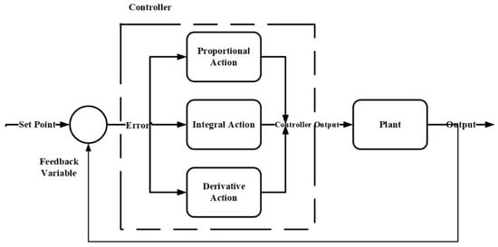
Figure 1. PID Diagram.
To guide a tractor through crop rows, Kodagoda combined a feed-forward controller with a fuzzy proportional derivative proportional integral controller [70]. They showed that their controller was insensitive to parameter uncertainty, load, and parameter fluctuations, and it could be implemented in real-time. In order to develop a closed-loop controller, Cortner used a PID implementation in the microcontroller, which was developed for the steering system of the AATV. Cortner found that the PID gains for the controller were P = (3/4), I = (1/2048), and D = 4 [71]. Eski and Kus used a PID controller in order to control a UAV. The results showed that there is an overshoot of 1 cm in 0.00001 s. After this point, the unit step signal was tracked with no overshoot [72]. Due to the fact that the autonomous vehicle modifies its speed according to the estimated size and type of the reference trajectory curves, Hossain used PID controllers in his study to maintain an optimal speed while following the given trajectory [73].
3.2.2. Fuzzy Logic
Fuzzification, fuzzy inference, and defuzzification are the three steps of fuzzy logic control. Fuzzification transforms crisp input values into fuzzy ones. By applying fuzzy IF-THEN rules and logical operations, fuzzy values are mapped to different fuzzy values. Mamdani and Sugeno [74] are two types of fuzzy inference systems. Systems of all types are classified as Mamdani types, while dynamic nonlinear systems are classified as Sugeno types. In the defuzzification process, the linguistic output values from the previous step are aggregated. After the defuzzification process is completed, a single crisp value is produced as an outcome (Figure 2).
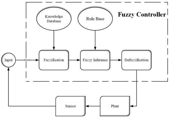
Figure 2. Fuzzy Logic Control (FLC) Diagram.
Using many-valued fuzzy logic (FL), Sumarsono built an ATV control system using GPS data [75]. To obtain useful data for hardware implementation, a fuzzy logic controller (FLC) simulation model was developed. To determine the radius and speed of the vehicle, the FLC used two inputs: the vehicle heading and the offset from the planned path. Expert experience and knowledge were FLC’s control knowledge base, and the center of gravity for singletons (CoGS) was used for defuzzification [75]. In addition, Sumarsono showed that the accuracy of FLC is dependent on the determination of membership functions [75]. In the membership functions of heading, offset, steering angle, radius, and speed, the appropriate numbers were set to 5, 5, 7, 7, and 3. Based on the constructed kinematic bicycle model of a tractor and implement, a fuzzy logic-based controller was proposed to automatically steer an implement using hydraulic cylinder actuators to cover crop fields [76]. To navigate in agricultural environments, Bonadies and others [77] applied PID and fuzzy controllers to an unmanned ground vehicle. Agricultural produce and ground are differentiated from an image obtained from the camera. Within the image, the left and right boundaries of the crops and the center of the row were identified. The average percent overshoot for the fuzzy controller was 45.75%. The average velocity was 35.26 rpm, with a velocity standard deviation of 0.32 rpm and an absolute average error of 28.37. In his study, he found that fuzzy logic and PID controllers performed similarly [77]. Using an improved fuzzy logic control method, Yao and others [78] generated optimal steering angles for a wheeled autonomous vehicle to track a sequence of waypoints. In developing the path-tracking algorithm, accuracy, stability, and convergence speed were considered. The proposed IFM provides higher accuracy, stability, and convergence speed when compared with conventional fuzzy logic control [78].
3.2.3. Genetic (Evolutionary) Algorithms
A genetic algorithm (GA) is a global, parallel search and optimization method that uses a population of potential solutions to solve a problem. Within the population, each individual represents a particular solution to the problem, which is usually encoded in genetic code. Over generations, the population evolves to produce better solutions to the problem. GA are efficient and appropriate optimization methods for control system design [79] for both feedback controllers and feedforward controllers.
GA’s operational principle is based on natural selection to select better-fit solution candidates and to generate the most-fit solution by using crossover operations and very limited artificial mutation operations. A genetic algorithm is a method of solving optimization and search problems using true or approximate solutions. Inheritance, mutation, selection, and crossover are techniques that are inspired by biological evolution. Gas was used by Ryerson and Zhang to plan a guided vehicle’s optimal path [81]. They found that the total coverage achieved was greater than 90% on four of the eight runs. There was an average coverage of 89%. Several combinations of lateral and heading deviations were tested by Ashraf using genetic algorithms [82]. According to their finding for vehicles moving along sloped land, the mean and standard deviation of lateral deviation along contour directions were 0.047 m and 0.039 m, respectively, which are highly insignificant. Shiltagh and Jalal used a modified genetic algorithm (MGA) developed for global path planning, and the application of MGA to the problem of navigation was investigated under the assumption that a model of the environment had been developed [83]. The simulation results demonstrated that this algorithm had a great potential to solve path planning with satisfactory results in terms of minimizing distance and execution time, and it was also determined that 374.47 s were required to find the shortest generated path (distance) with a length of 30.86 m [83]. In another similar study to Shiltagh research, the genetic algorithm used the grid method to mark the geographical environment information and map the environmental information to the grid [84]. According to the algorithm in this entry, mutation probability had the greatest impact on the effective path ratio. According to the study, when the mutation probability is 0.09, the effective path ratio is 80.65%. Furthermore, the effective path ratio remained approximately 80%, regardless of how the population size, evolutionary algebra, and crossover probability were selected.
3.2.4. Artificial Neural Network
Typically, neural networks consist of three layers: input, hidden, and output (Figure 3). One or more layers could make up the hidden layer, depending on the requirements. Adaptations were made to the neural networks to compensate for inclinations and magnetism errors. Prior to performing the main maneuvers, it was necessary to train the neural network and the AATV. Due to the hidden layers in neural networks, one of the major disadvantages was the use of unidentified boxes (so-called black boxes) in programming. In order to explain the input-output relationship of vehicle motion on sloping land, Torisu developed a neural network (NN) vehicle model rather than a dynamic or kinematic model [85]. In a comparison of experiments and simulations of vehicle motion in slope-land environments, Zhu found that the NN model was suitable to represent the input-output relationship of vehicle motion. Also, the NN vehicle model was deemed suitable for representing the tractor’s motion on sloping terrain for autonomous navigation [76]. Eski and Kus showed that the unmanned agricultural vehicles with a model-based neural network PID control system followed the given reference trajectory with minimum errors in formidable road conditions and that they reduced overshoot to a considerable extent [72]. A neural network’s backpropagation algorithm is probably its most fundamental component. A chain rule algorithm is used to train neural networks effectively. The backpropagation method performs a backward pass through a network after each forward pass while adjusting the model’s parameters (weights and biases). By using the back propagation algorithm, Ashraf developed a NN vehicle model for sloped terrain conditions. In order to generalize the optimal steering for different land slopes, Ashraf developed a model that utilizes an NN-based steering controller. With a prototype test tractor, he conducted autonomous travel tests on sloping lands and found that the tractor could follow predetermined rectangular paths precisely [82]. As a result of his study, the average lateral deviations were only 0.058 m and 0.063 m for the four rectilinear motions, whereas the average heading angles were 2.950 and 1.935, both of which are insignificant for tractor motion even on flat terrain.
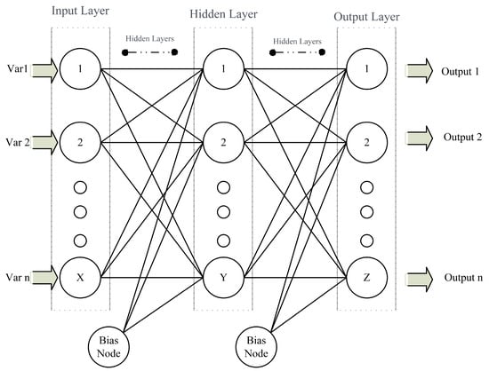
Figure 3. Neural network schema.
3.2.5. MPC
MPC consists of predicting the future behavior of the controlled system over a finite time horizon and computing an optimal control input that maximizes a priori-defined functional cost while satisfying the system constraints. For a more precise calculation of the control input, an optimal open-loop control problem of finite horizon is solved at each sampling instant. After applying the first part of the optimal input trajectory to the system, the horizon is shifted, and the process is repeated. As a result of its ability to explicitly incorporate a performance criterion and hard state constraints into its design, MPC is particularly successful (Figure 4).
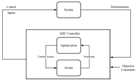
Figure 4. MPC Basic Control Loop.
Multivariate, complex, and unpredictable are the characteristics of agricultural systems [86]. Traditionally, control technologies such as on/off, P, and PID are easy to implement, but they cannot control time-delayed processes [87,88]. In addition, adjustment of the controller takes considerable time and effort [89]. In the past few decades, MPC has been extensively investigated as a promising control strategy [90,91,92,93] and has also been applied in the industrial sector [94]. There are a few alternative versions of the MPC algorithm used in autonomous vehicle control, e.g., a prescribed performance control algorithm proposed to establish accurate tracking control for a tractor trailer [95]. A combine harvester was controlled using constraint MPC and an alternative ASM as part of the cruise control process [96]. A navigation task was completed by Backman using NMPC. It is necessary to have sufficient accuracy for lateral errors of up to 10 cm at 12 km/h [97]. It is also possible to use the MPC for inland navigation in addition to the navigation of agricultural machines [98]. It is extremely difficult to control path-tracking in agriculture because there are so many complex bodies involved. Using NMHE and rapid distributed nonlinear MPC, Kayacan developed an estimation scheme for the state and parameters of the system [99]. As part of the path-tracking error control of unmanned ground vehicles, linear MPC was designed, resulting in an average Euclidian distance error of 23.49 cm and 21.21 cm on straight lines, respectively, while the average Euclidian distance error was 39.82 cm and 36.21 cm on curved lines. LMPC calculates in approximately 1.1 ms, which is faster than NMPC [48]. Based on an mp-MIQP technique, Yang presented explicit MPC for the reduction of trailer tracking errors and smoothing tractor steering angle behavior [100]. MPC outperformed LQC in tracking multivariate systems under constraints, according to Yakub [101]. A high-precision closed-loop tracking method based on LTV-MPC has been proposed by Plessen. Precision tracking is possible within millimeters [102]. Additionally, MPC could be used to track the path of hydraulic forestry cranes in forests [103,104]. MPC uses a model to predict and optimize the steering angle and velocity of an AV, as well as other features of the process. To overcome the shortcomings of PID, ANN, and other similar controllers, different types of MPC were developed, such as hybrid MPC, robust MPC, adaptive MPC, nonlinear MPC, tube-based MPC, distributed MPC, stochastic MPC, and explicit MPC [105]. The MPC controller can be used for a number of reasons, including: (1) MPCs are capable of handling MIMO systems in the same way as ANNs. It is useful when inputs and outputs are predicted to have some interaction. A prediction model, a rolling optimization, and feedback adjustments are all involved in the MPC. In MPC, the outputs are controlled simultaneously by a multivariable controller, which takes into account all variables within a system. (2) As AVs violate constraints, they will have unwanted consequences, which can be handled by MPC. There should be a safe distance between autonomous vehicles and obstacles, and multi-robot systems should follow speed limits. The acceleration limits of AVs are also a limitation. An MPC algorithm should track a desired trajectory if all these constraints are met. In the MPC, previewing is like feedback control. In the event that the controller is unaware that a corner is approaching, the AV can only apply its brake during cornering when it is traveling on a curve or turning at the headland. AVs with safety sensors, such as cameras that provide trajectory information, will provide information to the controller ahead of the upcoming corner. As a result, it is able to brake sufficiently so that it can stay on the road safely. Control performance can be improved by incorporating future reference information into the MPC.
3.2.6. Kalman Filter
Digital control engineering is one area in which the Kalman filter (KF) is frequently used. Control engineers use the filter to eliminate measurement noise that may interfere with the performance of a system under control. Additionally, it provides an estimate of the current state of the process or system. The KF is used (1) to estimate future position and velocity based on the current position of objects or people. (2) To estimate the state, position, and velocity of a vehicle, navigation systems use the output of an inertial measurement unit (IMU) and a global navigation satellite system (GNSS) receiver. (3) To feature tracking or cluster tracking applications based on computer vision. The KF process has two steps: 1. Prediction step: Based on previous measurements, the KF predicts the system’s next state. 2. Update step: KF calculates the system’s current state based on measurements taken at that time.
Multi-sensor data fusion is based on the KF, which offers a solid theoretical framework. The approach relies on tracking the vehicle’s location at all times or the system’s state. INS and GPS need to be integrated using Kalman filters in a highly dynamic system that is likely to experience significant acceleration. When the GPS signal is lost, these integrated systems can provide short-term positioning information that is reliable. A wide range of literature exists on integrating INSs with GPSs and/or other sensors [107,108,109,110]. KF was applied to draw DGPS measurements and effectively reduce the RMS positioning error by removing DGPS noise [111]. Using a bandpass filter and extended KF, Hague and Tillett combined image processing with bandpass filtering [112]. A new sigma-point filter has been proposed in order to improve the KF performance [113]. Based on simulations, Zhang found that the sigma-point Kalman filter had better numerical robustness and computational efficiency [114]. By considering ATVs’ multiple positioning systems and comparing them, Pratama uses the Extended Kalman Filter (EKF) to detect abnormal deviations. Based on residue values, their model can detect one fault condition at a time [115]. An innovative, robust CKF with a scaling factor was presented by Gao in his study. The Mahalanobis distance criterion is used to identify abnormal observations. An increased observation noise covariance was achieved by adding a robust factor (scaling factor) to the standard CKF by using the Mahalanobis distance criterion. This results in a decrease in filtering gain when abnormal observations are present. In addition to improving the robustness of CKF, the proposed solution does not depend on abnormal observations to influence navigation solutions [116]. GPS-based navigation was developed that allowed an autonomous ATV to follow a virtual path in the field [32]. Their ATV was equipped with an EPS, PID, low-level servo controller, and high-level controller based on the estimation algorithm, EKF. The position data was obtained by an RTK global navigation satellite system and used to precisely turn the EPS motor on the ATV’s steering shaft [32].
3.2.7. Machine Learning: DRL
Reinforcement learning (RL). Machine learning techniques such as reinforcement learning reward and/or punish desired behaviors. There are two types of RL methods: model-free and model-based. An approach based on value-based model-free learning takes a state and action as inputs and outputs the value. By selecting the action that maximizes the value function, the policy is extracted. An approach based on models learns a predictive function from the current state and a sequence of actions to predict the future state. Utilizing predicted future states, policies are extracted by selecting actions that maximize future rewards. A model-free algorithm is capable of learning complex tasks [117]; however, they are typically sample-inefficient, as opposed to model-based algorithms, which are sample-efficient but difficult to scale to complex, high-dimensional tasks. Reinforcement learning agents are capable of interpreting their environment, taking actions, and learning through trial and error. RL focuses on the problem of goal-directed agents interacting with uncertain environments, which is crucial for navigating rough terrain in unknown conditions.
Deep-reinforcement learning (DRL) has been incredibly successful since its introduction [118]. Particularly, DRL has found a niche in robotic manipulation based on vision. It has been shown that robots controlled by neural networks with DRL-trained representations can solve complex tasks even in unstructured environments without requiring imitation learning. DRL-based local navigation of unknown rough terrain was presented by Josef and Degani. In comparison with traditional local planning methods, their method reduced planning time and improved planning success rates. In a goal-directed task, they used reward shaping to provide a dense reward signal [119]. With Kahn’s algorithm, robot navigation policies can be learned in a self-supervised manner that requires minimal human interaction, using samples in an efficient, stable, and high-performing manner [120]. Deep RL is capable of learning control for rough terrain vehicles that have continuous, high-dimensional observations and actions in their environment, according to Wiberg [121].
A comparison analysis of control algorithms for AATVs is shown in Table 1, which shows the advantages and disadvantages of commonly used control algorithms.
Table 1. Comparison of commonly used algorithms of AATVs.
| Control Method | Advantages | Disadvantages | References |
|---|---|---|---|
| Fuzzy |
|
|
[74,75,76,77,78,79] |
| GA |
|
|
[79,80,81,82,83,84] |
| ANN |
|
|
[72,76,82,85] |
| MPC |
|
|
[86,87,88,89,90,91,92,93,94,95,96,97,98,99,100,101,102,103,104,105] |
| ML: DRL |
|
|
[117,118,119,120,121] |
| PID |
|
|
[70,71,72,73] |
| Kalman filter |
|
|
[106,107,108,109,110,111,112,113,114,115,116] |
Information
Subjects:
Agricultural Engineering
Contributors
MDPI registered users' name will be linked to their SciProfiles pages. To register with us, please refer to https://encyclopedia.pub/register
:
View Times:
521
Revision:
1 time
(View History)
Update Date:
21 Feb 2024
Table of Contents


Notice
You are not a member of the advisory board for this topic. If you want to update advisory board member profile, please contact office@encyclopedia.pub.
OK
Confirm
Only members of the Encyclopedia advisory board for this topic are allowed to note entries. Would you like to become an advisory board member of the Encyclopedia?
Yes
No
${ textCharacter }/${ maxCharacter }
Submit
Cancel
Back
Comments
${ item }
|
${ item.createdUser.fullName }
${ item.createdAt }
${ item.vote }
${ item.reply }
Delete
${ reply.createdUser.fullName }
${ reply.createdAt }
${ reply.vote }
Delete
There is no reply to this comment~
${ item.replyTextCharacter }/${ item.replyMaxCharacter }
Submit
Cancel
More
No more~
There is no comment~
${ textCharacter }/${ maxCharacter }
Submit
Cancel
${ selectedItem.replyTextCharacter }/${ selectedItem.replyMaxCharacter }
Submit
Cancel
Confirm
Are you sure to Delete?
Yes
No