Your browser does not fully support modern features. Please upgrade for a smoother experience.
Submitted Successfully!
 +1 credit
Thank you for your contribution! You can also upload a video entry or images related to this topic.
For video creation, please contact our Academic Video Service.
| Version | Summary | Created by | Modification | Content Size | Created at | Operation |
|---|---|---|---|---|---|---|
| 1 | Omar El Seoud | -- | 1595 | 2024-01-13 00:08:53 | | | |
| 2 | Rita Xu | -5 word(s) | 1590 | 2024-01-15 03:35:20 | | |
Video Upload Options
We provide professional Academic Video Service to translate complex research into visually appealing presentations. Would you like to try it?
Cite
If you have any further questions, please contact Encyclopedia Editorial Office.
El Seoud, O.A.; Possidonio, S.; Malek, N.I. Solvatochromism in Solvent Mixtures. Encyclopedia. Available online: https://encyclopedia.pub/entry/53790 (accessed on 22 July 2026).
El Seoud OA, Possidonio S, Malek NI. Solvatochromism in Solvent Mixtures. Encyclopedia. Available at: https://encyclopedia.pub/entry/53790. Accessed July 22, 2026.
El Seoud, Omar A., Shirley Possidonio, Naved I. Malek. "Solvatochromism in Solvent Mixtures" Encyclopedia, https://encyclopedia.pub/entry/53790 (accessed July 22, 2026).
El Seoud, O.A., Possidonio, S., & Malek, N.I. (2024, January 13). Solvatochromism in Solvent Mixtures. In Encyclopedia. https://encyclopedia.pub/entry/53790
El Seoud, Omar A., et al. "Solvatochromism in Solvent Mixtures." Encyclopedia. Web. 13 January, 2024.
Copy Citation
Many reactions are carried out in solvent mixtures, mainly because of practical reasons. For example, E2 eliminations are favored over SN2 substitutions in aqueous organic solvents because the bases are desolvated.
binary solvent mixtures
solvatochromism
solvatochromic probes
solvation models
1. Reasons for Using Mixed Solvents in Chemistry
Solvent mixtures are extensively employed in chemistry for practical reasons. For example, the solubilities of inorganic bases, such as KOH, and other electrolytes in alcohols are enhanced in presence of water [1][2]. Cellulose that is insoluble in water is, however, readily soluble in some aqueous electrolyte solutions [3], water-DMSO mixtures [4], and mixtures of ionic liquids-molecular solvents (ILs-MSs) [5][6][7][8]. In the latter example, cellulose dissolution is attributed to the disruption of the strong hydrogen-bonding (H-bonding) between the hydroxyl groups of the anhydroglucose units, as well as to the hydrophobic interactions between cellulose chains, as shown in Figure 1a (IL-DMSO). Consequently, addition of protic non-solvents to solutions of cellulose in IL-MS causes biopolymer precipitation because the non-solvent efficiently solvates the ions of the IL (Figure 1b).

Figure 1. (a) A simplified scheme for cellulose dissolution in ionic liquid-DMSO. The biopolymer dissolution is attributed to interactions of its hydroxyl groups with the ions of the ionic liquid and the dipole of DMSO. (b) Effects of the addition of a protic non-solvent (such as water or ethanol) on the dissolution of cellulose IL-dipolar solvent. Addition of the non-solvent leads to cellulose precipitation.
In addition to enhanced biopolymer solubility, the use of mixed solvents also causes noticeable changes in the physicochemical properties, such as a reduction in viscosity, leading to better heat and mass transfer, as shown by Figure 2a,c.

Figure 2. (a) Dependence of the viscosity (η) of PEG 400-DMSO on the mole fraction of PEG 400 at different temperatures: ◼, 25 °C; ●, 30 °C; ▲, 35 °C; ▼, 40 °C; ⧫, 45 °C; ◄, 50 °C. (b) Viscosities of BuMeImCl-DMF (1-butyl-3-methylimidazolium chloride-N,N-Dimethylformamide) mixtures as a function of mole fraction of DMF: ■, 30 °C; □, 35 °C; ●, 40 °C; ○, 45 °C; ▲, 50 °C; △, 55 °C; ▼, 60 °C; ∇, 65 °C; ♦, 70 °C; ◊, 75 °C; ★, 80 °C. (c) Effects of increasing the mole fraction of DMSO (χS) on the viscosity of cotton cellulose in binary mixtures of DMSO with the ILs AlMeImCl (1-allyl-3-methylimidazolium chloride) and BuMeImCl. The insert is the logarithm-linear plot of the reduced viscosity ratio versus DMSO mole fraction at 25 °C.
2. A Rationale for Effects of Mixed Solvents on Chemical Phenomena
How do researchers explain these interesting and very useful effects of binary solvent mixtures on diverse chemical phenomena? While deceptively simple, this question cannot be answered in a straightforward manner. Consider, for example, the fact that most physicochemical properties of binary mixtures are not ideal. That is, the property of the binary mixture does not vary in a simple way as a function of binary solvent composition, as shown in Figure 3a–c.

Figure 3. (a) Density-based excess molar volumes as a function of mole fraction and temperature for PEG 400-DMSO. (a) ◼, 25 °C; ●, 30 °C; ▲, 35 °C; ▼, 40 °C; ⧫, 45 °C; ◄, 50 °C. (b) Deviation of viscosity of mixtures of BuMeImCl-DMF from the values calculated from Σ χcomponent × Vmolar volume of component. ■, 30 °C; □, 35 °C; ●, 40 °C; ○, 45 °C; ▲, 50 °C K; △, 55 °C; ▼, 60 °C; ∇, 65 °C; ♦, 70 °C; ◊, 75 °C; ★, 80 °C. (c) Excess molar volume (VE) of binary mixed systems for water-DMSO; water-MF, and DMSO-DMF at 25 °C.
The reason behind this non-ideality is clearly the interactions between components of the binary solvent mixture. To a first approximation, one expects that the composition of the solvation layer of a dissolved substance (which researchers will refer to as “probe”) should be the same as that of bulk binary mixture. Consequently, the same explanations given for bulk binary mixtures should apply to the solvation layers of the dissolved probes. This simple view, however, does not hold in most cases because probe-solvent nonspecific and specific interactions were not taken into consideration. These interactions change the composition of the solvation layers relative to bulk solvent mixtures, as shown below.
The composition of the solvation layer of a probe may deviate from that of an (already non-ideal) bulk solvent mixture due to the so-called “preferential solvation” of the probe by one component of the mixture (Figure 4). In principle, this phenomenon includes contributions from probe-independent “dielectric enrichment”, and probe-solvent interactions. The first mechanism is operative in mixtures of nonpolar/low polar solvents, such as cyclohexane-THF (Tetrahydrofuran). It denotes enrichment of the probe solvation layer (relative to that of bulk solvent mixture) by the component of larger dielectric constant (or relative permittivity), due to non-specific probe dipole-solvent dipole interactions [9][10][11].
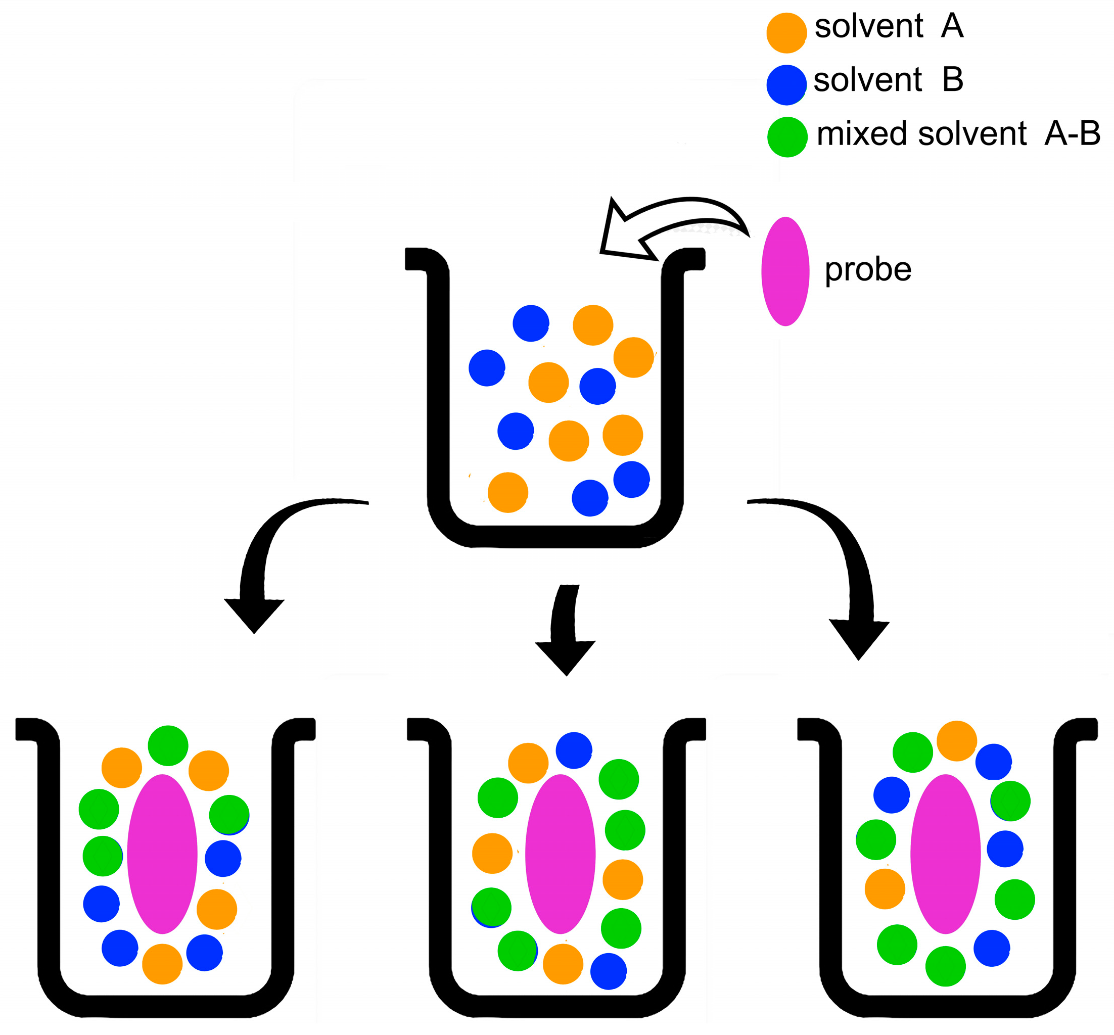
Figure 4. Schematic representation of the solvation of a solute in a binary solvent mixture composed of two solvents (A, B), and the “mixed” solvent A-B, whose formation is discussed below. The parts of the lower line represent from the left: ideal solvation, i.e., the composition of the probe solvation layer is the same as that of bulk solvent mixture; preferential solvation by the solvents (A, A-B); preferential solvation by the solvents (B, A-B).
The second solvation mechanism is dominant in protic solvents (such as aqueous alcohols) and their mixtures with strongly dipolar solvents (water-DMSO, alcohol-DMF, etc.). It is essentially due to solute-solvent H-bonding and hydrophobic interactions. One additional complication is that solvent-solvent H-bonding generates an additional or “mixed” solvent species that should be considered. For example, in mixtures of water (W) and alcohol (ROH), and W-DMSO, researchers have in solution both the parent and the mixed solvents, HOH…O(H)R and HOH…O(H)=S(CH3)2 [12]; this turns analysis of the solvation data more complex. In summary, most significant consequence of preferential solvation is that compositions of the solvation layers of most probes are different from those of the corresponding bulk solvent mixtures; these composition differences are probe-, and temperature-dependent [13][14].
How do researchers calculate the “effective” (or local) composition of the solvation layer of a probe? Several techniques were employed to solve this problem, including FTIR [15], resonance Raman spectroscopy [16], and X-ray diffraction (for solvated crystals) [17]. The most useful approach is to use solvatochromic indicators as models for the compounds of interest, e.g., reactants. Solvatochromic probes are substances whose absorption or emission spectra are sensitively dependent on the solvent or the composition of solvent mixtures (Figure 5). The reason for solvatochromism is that the energy difference between the probe’s ground and excited states is sensitively affected by probe-solvent interactions, leading to medium-dependent values of λmax, and hence a change in solution color. For most probes, the solvatochomism is negative, meaning there is a hypsochromic shift of the longest wavelength absorption band with increasing medium polarity. The reason is that solvents stabilize the zwitterionic ground state much more than the diradical excited state (see Figure 6 for light-induced transition of the probe t-Bu5RB). The latter corresponds to a so-called FranckCondon excited state, because the time scale of the electronic excitation (ca. 10−15 s) is much shorter than that required for the solvent molecule to reorient in order to stabilize the probe’s excited state. The energy of this transition furnishes the solvatochromic property of interest, vide infra.

Figure 5. Examples of solvatochromism. Part (a) is for MePMBr2 (2,6-dibromo-4-[(E)-2-(1-methylpyridinium-4-yl)ethenyl]) empirical polarity indicator in (from left) ethanol, water, acetone, and dichloromethane. Part (b) is that for the empirical polarity probe t-Bu5RB, Figure 6), in (mineral) diesel oil and its mixtures with 25, 50, 75% bioethanol, and in pure bioethanol, respectively. Part (c) shows the dependence of solution color on the structure of the solvatochromic probe. The structures and names of these probes are shown in Figure 7.
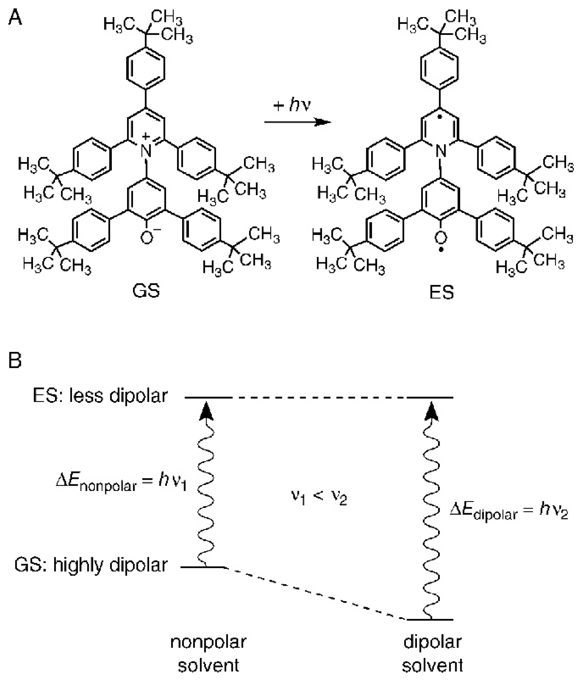
Figure 6. (A) The molecular structure of the solvatochromic indicator dye, t-Bu5RB (2,6-bis [4-(t-butyl)phenyl]-4-{2,4,6-tris[4-(t-butyl)phenyl]pyridinium-1-yl}phenolate): a zwitterionic pyridinium-N-phenolate betaine dye with a highly dipolar electronic ground state (GS) and a much less dipolar first excited state (ES). (B) A schematic qualitative representation of the solvent influence on the differences ΔE between the energies of the GS and ES of t-Bu5RB, dissolved in a nonpolar and a dipolar solvent, respectively.

Figure 7. Structures and acronyms of some solvatochromic probes, employed to calculate the solvent descriptors shown in Equation (1).
This approach was advanced thanks to the work of professor C. Reichardt, initially under the supervision of professor K. Dimroth at Marburg university [18][19]. The experimental part is relatively simple: register the UV-Vis spectrum of a solvatochromic probe → calculate the value of λmax of a specific peak (the longest wavelength, due to intermolecular charge-transfer within the probe) → use the value of λmax to calculate the desired property, or descriptor, of the solvent or solvent mixture. The power of solvatochromism is that it can be employed to calculate the overall (or empirical) solvent polarity scale, ET (in kcal/mol), as well as the individual solvent descriptors that contribute to ET, namely solvent Lewis acidity (SA), solvent Lewis basicity (SB), solvent dipolarity (SD), and solvent polarizability (SP), where S refers to solvent. Other abbreviations that were employed for designating these descriptors include SdP and SP for solvent dipolarity and polarizability, respectively. For consistency, however, researchers use two letters to designate each solvent descriptor.
Equation (1) shows the relationship of these solvent descriptors:
where ET(probe)0 corresponds to gas phase, the descriptors (SA, SB, SD, SP) are those defined above, and (a, b, d, and p) are the corresponding regression coefficients. Figure 7 shows some solvatochromic probes used to calculate the descriptors of Equation (1). In the Taft–Kamlet–Abboud approach, similar solvatochromic parameters and different symbols were employed to describe probe–solvent interactions, α, β, and π* for solvent Lewis acidity, Lewis basicity, and (combined) dipolarity/polarizability [20]. The signs of the coefficients in Equation (1) indicate whether the property of the solvent considered increases (positive sign) or decreases (negative sign) the empirical solvent polarity [21].
ET(probe) = ET(probe)0 + aSA + bSB + dSD + pSP
References
- Chiavone-Filho, O.; Rasmussen, P. Solubilities of Salts in Mixed Solvents. J. Chem. Eng. Data 1993, 38, 367–369.
- Pinho, S.P.; Macedo, E.A. Solubility of NaCl, NaBr, and KCl in Water, Methanol, Ethanol, and Their Mixed Solvents. J. Chem. Eng. Data 2005, 50, 29–32.
- Dogan, H.; Hilmioglu, N.D. Dissolution of cellulose with NMMO by microwave heating. Carbohydr. Polym. 2009, 75, 90–94.
- Kostag, M.; Jedvert, K.; Achtel, C.; Heinze, T.; El Seoud, O.A. Recent advances in solvents for the dissolution, shaping and derivatization of cellulose: Quaternary ammonium electrolytes and their solutions in water and molecular solvents. Molecules 2018, 23, 511.
- El Seoud, O.A.; Bioni, T.A.; Dignani, M.T. Understanding cellulose dissolution in ionic liquid-dimethyl sulfoxide binary mixtures: Quantification of the relative importance of hydrogen bonding and hydrophobic interactions. J. Mol. Liq. 2021, 322, 114848.
- Keppeler, N.; Pires, P.A.R.; Freitas, J.L.S.; El Seoud, O.A. Cellulose dissolution in mixtures of ionic liquids and molecular solvents: The fruitful synergism of experiment and theory. J. Mol. Liq. 2023, 386, 122490.
- Minnick, D.L.; Flores, R.A.; DeStefano, M.R.; Scurto, A.M. Cellulose Solubility in Ionic Liquid Mixtures: Temperature, Cosolvent, and Antisolvent Effects. J. Phys. Chem. B 2016, 120, 7906–7919.
- Zhong, C.; Cheng, F.; Zhu, Y.; Gao, Z.; Jia, H.; Wei, P. Dissolution mechanism of cellulose in quaternary ammonium hydroxide: Revisiting through molecular interactions. Carbohydr. Polym. 2017, 174, 400–408.
- Suppan, P. Local polarity of solvent mixtures in the field of electronically excited molecules and exciplexes. J. Chem. Soc. Faraday Trans. 1 Phys. Chem. Condens. Phases 1987, 83, 495.
- Suppan, P. Time-resolved luminescence spectra of dipolar excited molecules in liquid and solid mixtures. Dynamics of dielectric enrichment and microscopic motions. Faraday Discuss. Chem. Soc. 1988, 85, 173.
- LNovaki, P.; El Seoud, O.A. Solvatochromism in binary solvent mixtures: Effects of the molecular structure of the probe. Berichte Bunsenges. Phys. Chem. 1997, 101, 902–909.
- Skaf, M.S. Molecular Dynamics Study of Dielectric Properties of Water−Dimethyl Sulfoxide Mixtures. J. Phys. Chem. A 1999, 103, 10719–10729.
- El Seoud, O.A. Solvation in pure and mixed solvents: Some recent developments. Pure Appl. Chem. 2007, 79, 1135–1151.
- Machado, V.G.; Stock, R.I.; Reichardt, C. Pyridinium N -Phenolate Betaine Dyes. Chem. Rev. 2014, 114, 10429–10475.
- Bai, B.; Li, Z.; Wang, H.; Li, M.; Ozaki, Y.; Wei, J. Exploring the difference in xerogels and organogels through in situ observation. R. Soc. Open Sci. 2018, 5, 170492.
- McHale, J.L. Subpicosecond Solvent Dynamics in Charge-Transfer Transitions: Challenges and Opportunities in Resonance Raman Spectroscopy. Acc. Chem. Res. 2001, 34, 265–272.
- Jha, K.K.; Kumar, A.; Munshi, P. Solvatochromism and Reversible Solvent Exchange Phenomena in Solvatomorphic Organic Chromophore Crystals. Cryst. Growth Des. 2023, 23, 2922–2931.
- Dimroth, K.; Reichardt, C.; Siepmann, T.; Bohlmann, F. Über Pyridinium-N-phenol-betaine und ihre Verwendung zur Charakterisierung der Polarität von Lösungsmitteln. Justus Liebigs Ann. Chem. 1963, 661, 1–37.
- Reichardt, C.; Welton, T. Solvents and Solvent Effects in Organic Chemistry, 4th ed.; John Wiley & Sons: Hoboken, NJ, USA, 2011.
- NWeiß; Schmidt, C.H.; Thielemann, G.; Heid, E.; Schröder, C.; Spange, S. The physical significance of the Kamlet–Taft π * parameter of ionic liquids. Phys. Chem. Chem. Phys. 2021, 23, 1616–1626.
- El Seoud, O.A.; Kostag, M.; Jedvert, K.; Malek, N.I. Cellulose in Ionic Liquids and Alkaline Solutions: Advances in the Mechanisms of Biopolymer Dissolution and Regeneration. Polymers 2019, 11, 1917.
More
Information
Subjects:
Chemistry, Physical
Contributors
MDPI registered users' name will be linked to their SciProfiles pages. To register with us, please refer to https://encyclopedia.pub/register
:
View Times:
1.1K
Revisions:
2 times
(View History)
Update Date:
15 Jan 2024
Table of Contents


Notice
You are not a member of the advisory board for this topic. If you want to update advisory board member profile, please contact office@encyclopedia.pub.
OK
Confirm
Only members of the Encyclopedia advisory board for this topic are allowed to note entries. Would you like to become an advisory board member of the Encyclopedia?
Yes
No
${ textCharacter }/${ maxCharacter }
Submit
Cancel
Back
Comments
${ item }
|
${ item.createdUser.fullName }
${ item.createdAt }
${ item.vote }
${ item.reply }
Delete
${ reply.createdUser.fullName }
${ reply.createdAt }
${ reply.vote }
Delete
There is no reply to this comment~
${ item.replyTextCharacter }/${ item.replyMaxCharacter }
Submit
Cancel
More
No more~
There is no comment~
${ textCharacter }/${ maxCharacter }
Submit
Cancel
${ selectedItem.replyTextCharacter }/${ selectedItem.replyMaxCharacter }
Submit
Cancel
Confirm
Are you sure to Delete?
Yes
No