+1 credit
| Version | Summary | Created by | Modification | Content Size | Created at | Operation |
|---|---|---|---|---|---|---|
| 1 | Brittany S Barker | -- | 4032 | 2023-12-27 21:03:47 | | | |
| 2 | Lindsay Dong | Meta information modification | 4032 | 2023-12-28 02:38:05 | | | | |
| 3 | Brittany S Barker | Meta information modification | 4032 | 2023-12-29 16:32:53 | | |
Video Upload Options
Phenological maps can depict the development and seasonal activities (phenology) of invasive insects at area-wide scales, such as counties, states, or entire nations. When regularly updated using real-time and forecast climate data, these maps may improve the timeliness of early detection and control tactics that target specific life stages. Rapid responses to invasive insects may increase the likelihood that populations are eradicated or controlled before they can spread or increase in size. Phenological maps may also be used to assess pest establishment risk, investigate pest–host interactions, and measure climate-driven changes in pest phenology.
1. Introduction
2. Data Requirements for Degree-Day Models
3. Types of Phenological (Degree-Day) Maps
3.1. Generic Degree-Day Map
3.2. Degree-Day Lookup Table Map
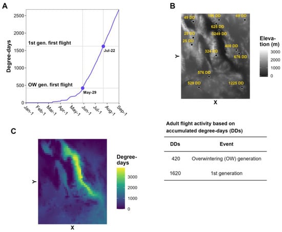
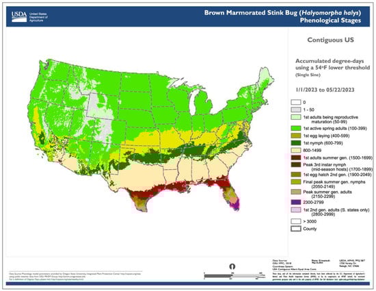
Degree-day lookup table maps show the current life stages or phenological events of an organism that correspond to specified values or ranges of accumulated degree-days for a specified date (Figure 3). Thus, degree-day accumulations, which are depicted in generic degree-day maps, are matched to specific points or events during the life cycle. For insects, life cycle points (and events) could typically include the egg stage present, egg hatch, larval stage present, pupal stage present, adult emergence and presence, and egg laying. The simplicity of the approach and its applicability to multiple organisms has sustained its use for several years.
-
A relatively straightforward workflow. The workflow of generating a degree-day lookup table map involves using gridded daily Tmin and Tmax data to calculate degree-day accumulations between a start date (usually 1 January, although some models use other start dates, such as 1 March) and a specified end date. Degree-day lookup tables are then used to associate degree-day accumulations with life stages, and output maps depict the results with color tables and legends.
-
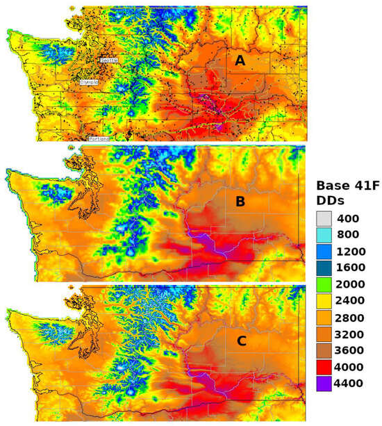
The use of common base thresholds for multiple species. As degree-day lookup table maps are relatively simple and generic, there is the potential to use the same lower temperature threshold base maps for multiple species. This contrasts with more complex models that would require a separate base map for each case because of the application of different parameter values, including lower and upper thresholds, calculation methods, start dates, or diapause. The use of upper thresholds is relatively rare, at least for degree-day lookup table maps. For example, the SAFARIS FO Weekly maps produced by models for the old world bollworm [Helicoverpa armigera (Hübner)] and brown marmorated stink bug [Halyomorpha halys (Stål)] are constructed using the same 54 °F base maps, with no upper threshold.
-
An ability to provide a “snapshot in time” for a single date. This allows, for example, regular updates that provide a gradually changing view of the current or near-future status of insect phenology. For example, degree-day lookup table maps produced by the Degree-Day, establishment Risk, and Phenological event maps (DDRP) platform [16] every 2−3 days depict the life stage and generation of insects on the map issue date. The USA National Phenology Network’s Pheno Forecast maps take advantage of 7-day National Digital Forecast Database (NDFD) forecasts to provide a 1-week “look ahead” prediction for CONUS [49]. SAFARIS PestCAST maps include a 1-month forecast using a 7-day NDFD forecast followed by three weeks of recent 20-year average PRISM data [15].
-
Relatively simple design requirements. Degree-day lookup table maps can be designed as very simple visualization tools, such as by designing legend items to display only the stage or activity of interest (e.g., adult flight or egg hatch). Other stages and activities can then be represented as merged entries. The practice of focusing end users on a single target event represents a clear trade-off in reducing complexity (of multiple life stages) for users who may need clear directions in implementing surveillance or management actions.
3.3. Phenological Event Map
-
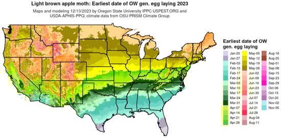
Standardization. Mapping dates of phenological events allows for the standardization of legends and color tables across multiple species and events. For example, the colors assigned to each range of dates in the legend (e.g., 1–8 January = dark blue, 9–16 January = medium blue, etc.) can be applied to several events within a species, as well the same or different events in other species. As an example, Figure 4 shows a phenological event map produced by DDRP that depicts the average date of egg laying by the overwintering generation of the light brown apple moth [Epiphyas postvittana (Walker)] for 2023.
-
Operationally ready. Phenological event maps could be considered a more operational (tactical) product than degree-day lookup tables because they predict dates of events for a particular life stage, potentially up to weeks or months into the future.
-
Simpler comparisons and expression of error rates. Phenological event maps allow for more direct comparisons of year-to-year variations of events than generic degree-day and degree-day lookup table maps. It is a relatively simple recordkeeping and reporting exercise to express differences in dates in the form of days difference [12][27][28]. This approach can also be used to express errors between predicted and observed events as discussed below (“8. Model validation”).
4. Applications of Phenological Maps
Phenological maps can support pest managers in timing treatments or other control tactics that target certain life stages. For example, phenological maps of egg hatch and larval development for the spongy moth were developed to support the timing of insecticidal sprays conducted for “stop the spread” programs in the eastern United States [30][31][32].
5. Gridded Climate Data
Maps used for within-season decision support of invasive insects depend on having access to real-time daily Tmin and Tmax data with spatial resolutions that are appropriate for the needs of decision-makers. For example, phenological maps at a 4 km resolution are generally sufficient to support pest surveillance programs for the entire CONUS [15], but are probably not appropriate for smaller scales, such as a county or city. Real-time PRISM data with a spatial resolution of 4 km are freely available, and higher resolution (800 m) data can be purchased from the PRISM group. Real-time DDRP forecasts at USPest.org are produced using PRISM data (4 km resolution) as climatic inputs, whereas monthly updated North America Multi-Model Ensemble (NMME) 7-month forecasts or recent 10-year average PRISM data (calculated on a bimonthly basis) are used to predict pest phenology up to the end of the year [16].
Phenological mapping for within-season decision support in areas outside of the United States is typically hindered by a lack of real-time gridded daily Tmin and Tmax data. However, historical datasets may be used for model development and validation, such as those for Europe [69], continental North America and Hawaii [70][71], Brazil [72][73], China [74][75], India [76], and Bangladesh, Nepal, and Pakistan [77].
Some phenological mapping studies overcame an absence of readily available gridded daily climate data by interpolating weather station data over a landscape of interest using custom software [31][50][78][79][80][81][82]. For example, the GEO-BUG platform offered four automated interpolation methods to map the date at which a pest insect species reached a specified life stage in the United Kingdom [78][80]. Interpolation methods commonly applied to Tmin and Tmax estimates include those based on distance analyses (e.g., inverse distance weighted and spline interpolation) or geostatistics (e.g., kriging and multiple regression) [33][47][80][81][82][83].6. Potential Sources of Error and Uncertainty
7. Increasing Model Realism While Maintaining Simplicity
8. Model Validation
9. Conclusions
References
- Bowers, J.H.; Malayer, J.R.; Martínez-López, B.; LaForest, J.; Bargeron, C.; Neeley, A.D.; Coop, L.; Barker, B.S.; Mastin, A.J.; Parnell, S.; et al. Surveillance for early detection of high-consequence pests and pathogens. In Tactical Sciences for Biosecurity of Animal and Plant Systems; Cardwell, K.F., Bailey, K.L., Eds.; IGI Global: Hershey, PN, USA, 2022; pp. 120–177.
- Reaser, J.K.; Veatch, S.D.; Burgiel, S.W.; Kirkey, J.; Brantley, K.A.; Burgos-Rodri, J. The early detection of and rapid response (EDRR) to invasive species: A conceptual framework and federal capacities assessment. Biol. Invasions 2020, 22, 1–19.
- Vänninen, I. Advances in Insect Pest and Disease Monitoring and Forecasting in Horticulture; Burleigh Dodds Science Publishing: Sawston, UK, 2022.
- Wilson, L.T.; Barnett, W.W. Degree-days: An aid in crop and pest management. Calif. Agric. 1983, 37, 4–7.
- Herms, D.A. Using degree-days and plant phenology to predict pest activity. In IPM (Integrated Pest Management) of Midwest Landscapes, Minnesota Agricultural Experiment Station Publication SB-07645; Krischik, V., Davidson, J., Eds.; Minnesota Agricultural Experiment Station: St. Paul, MN, USA, 2004; pp. 49–59.
- Ascerno, M.E. Insect phenology and integrated pest management. J. Arboric. 1991, 17, 13–15.
- Zalom, F.G.; Goodell, P.B.; Wilson, L.T.; Barnett, W.W.; Bentley, W.J. Degree-Days: The Calculation and Use of Heat Units in Pest Management; University of California, Division of Agriculture and Natural Resources: Berkeley, CA, USA, 1983.
- Gage, S.H.; Whalon, M.E.; Miller, D.J. Pest event scheduling system for biological monitoring and pest management. Environ. Entomol. 1982, 11, 1127–1133.
- Ferguson, A.W.; Skellern, M.P.; Johnen, A.; Richthofen, V.; Watts, N.P.; Bardsley, E.; Murray, A.; Cook, S.M. The potential of decision support systems to improve risk assessment for pollen beetle management in winter oilseed rape. Pest Manag. Sci. 2016, 72, 609–617.
- Jones, V.P.; Brunner, J.F.; Grove, G.G.; Petit, B.; Tangren, G.V.; Jones, W.E. A web-based decision support system to enhance IPM programs in Washington tree fruit. Pest Manag. Sci. 2010, 66, 587–595.
- Rossi, V.; Sperandio, G.; Caffi, T.; Simonetto, A.; Gilioli, G. Critical success factors for the adoption of decision tools in IPM. Agronomy 2019, 9, 710.
- Cormier, D.; Chouinard, G.; Pelletier, F.; Vanoosthuyse, F.; Joannin, R. An interactive model to predict codling moth development and insecticide application effectiveness. IOBC-WPRS Bull. 2016, 112, 65–70.
- Jones, V.P. Using phenology models to estimate insecticide effects on population dynamics: Examples from codling moth and obliquebanded leafroller. Pest Manag. Sci. 2021, 77, 1081–1093.
- Roltsch, W.J.; Zalom, A.G.; Strand, J.F.; Pitcairn, M.J.; Frank, J.R.; Ann, G.Z.; Strand, J.F.; Pitcairn, M.J. Evaluation of several degree-day estimation methods in California climates. Int. J. Biometeorol. 1999, 42, 169–176.
- Takeuchi, Y.; Tripodi, A.; Montgomery, K. SAFARIS: A spatial analytic framework for pest forecast systems. Front. Insect Sci. 2023, 3, 1198355.
- Barker, B.S.; Coop, L.; Wepprich, T.; Grevstad, F.S.; Cook, G. DDRP: Real-time phenology and climatic suitability modeling of invasive insects. PLoS ONE 2020, 15, e0244005.
- Coop, L.B.; Barker, B.S. Advances in understanding species ecology: Phenological and life cycle modeling of insect pests. In Integrated Management of Insect Pests: Current and Future Developments; Kogan, M., Heinrichs, E., Eds.; Burleigh Dodds Science Publishing: Sawston, UK, 2020; pp. 43–96.
- Welch, S.M.; Croft, B.A.; Brunner, J.F.; Michels, M.; Welch, B.; Croft, J.; Brunner, M.; Michels, S.M. PETE: An extension phenology modeling system for management of multi-species pest complex. Environ. Entomol. 1978, 7, 482–494.
- Nietschke, B.S.; Magarey, R.D.; Borchert, D.M.; Calvin, D.D.; Jones, E. A developmental database to support insect phenology models. Crop Prot. 2007, 26, 1444–1448.
- Orlandini, S.; Magarey, R.D.; Woo Park, E.; Sporleder, M.; Kroschel, J. Methods of agroclimatology: Modeling approaches for pests and diseases. In Agroclimatology: Linking Agriculture to Climate, Agronomy Monograph 60; Hatfield, J.H., Sivakuma, M.V.K., Prueger, J.H., Eds.; Wiley: Hoboken, NJ, USA, 2018; pp. 453–488. Available online: https://acsess.onlinelibrary.wiley.com/doi/book/10.2134/agronmonogr60 (accessed on 18 December 2023).
- Arnold, C.Y.Y. Maximum-minimum temperatures as a basis for computing heat units. Proc. Soc. Hortic. Sci. 1960, 76, 682–692.
- Wang, J.Y. A critique of the heat unit approach to plant response studies. Ecology 1960, 41, 785–790.
- Chuine, I.; Régnière, J. Process-based models of phenology for plants and animals. Annu. Rev. Ecol. Evol. Syst. 2017, 48, 159–182.
- Mirhosseini, M.A.; Fathipour, Y.; Reddy, G.V.P.R. Arthropod development’s response to temperature: A review and new software for modeling. Ann. Entomol. Soc. Am. 2017, 110, 507–520.
- Knight, A.L. Adjusting the phenology model of codling moth (Lepidoptera: Tortricidae) in Washington State apple orchards. Environ. Entomol. 2007, 36, 1485–1493.
- Brunner, J.F.; Hoyt, S.C.; Wright, M.A. Codling Moth Control—A New Tool for Timing Sprays; Cooperative Extension Bulletin, 1072; Washington State University: Pullman, WA, USA, 1987.
- Barros-Parada, W.; Knight, A.L.; Fuentes-Contreras, E. Modeling codling moth (Lepidoptera: Tortricidae) phenology and predicting egg hatch in apple orchards of the Maule Region, Chile. Chil. J. Agric. Res. 2015, 75, 57–62.
- Jorgensen, C.D.; Martinsen, M.E.; Westover, L.J. Validating Michigan State University’s codling moth model (MOTHMDL) in an arid environment. Gt. Lakes Entomol. 1979, 12, 203–212.
- Song, Y.H.; Coop, L.B.; Omeg, M.; Rield, H. Development of a phenology model for predicting Western cherry fruit fly, Rhagoletis indifferens Curran (Diptera: Tephritidae), emergence in the mid Columbia area of the western United States. J. Asia. Pac. Entomol. 2003, 6, 187–192.
- Régnière, J.; Sharov, A. Phenology of Lymantria dispar (Lepidoptera: Lymantriidae), male flight and the effect of moth dispersal in heterogeneous landscapes. Int. J. Biometeorol. 1998, 41, 161–168.
- Régnière, J.; Sharov, A. Simulating temperature-dependent ecological processes at the sub-continental scale: Male gypsy moth flight phenology as an example. Int. J. Biometeorol. 1999, 42, 146–152.
- Schaub, L.P.; Ravlin, F.W.; Gray, D.R.; Logan, J.A. Landscape framework to predict phenological events for gypsy moth (Lepidoptera: Lymantriidae) management programs. Environ. Entomol. 1995, 24, 10–18.
- Russo, J.M.; Liebhold, A.M.; Kelley, J.G.W. Mesoscale weather data as input to a gypsy moth (Lepidoptera: Lymantriidae) phenology model. J. Econ. Entomol. 1993, 86, 838–844.
- Foster, J.R.; Townsend, P.A.; Mladenoff, D.J. Mapping asynchrony between gypsy moth egg-hatch and forest leaf-out: Putting the phenological window hypothesis in a spatial context. For. Ecol. Manag. 2013, 287, 67–76.
- Samietz, J.; Graf, B.; Höhn, H.; Schaub, L.P.; Höpli, H.U. SOPRA: Forecasting tool for fruit tree pest insects. Rev. Suisse Vitic. Arboric. Hortic. 2007, 39, 187–194.
- Delahaut, K. Insects. In Phenology: An Integrative Environmental Science; Schwartz, M., Ed.; Kluwer Academic Publishers: Dordrecht, The Netherlands, 2003; pp. 405–419.
- Damos, P.T.; Savopoulou-Soultani, M. Temperature-driven models for insect development and vital thermal requirements. Psyche 2012, 2012, 123405.
- Pruess, K.P. Degree-day methods for pest management. Environ. Entomol. 1983, 12, 613–619.
- Campbell, A.; Frazer, B.D.; Gilbert, N.; Gutierrez, A.P.; Mackauer, M. Temperature requirements of some aphids and their parasites. J. Appl. Ecol. 1974, 11, 431–438.
- Rebaudo, F.; Rabhi, V.B. Modeling temperature-dependent development rate and phenology in insects: Review of major developments, challenges, and future directions. Entomol. Exp. Appl. 2018, 166, 607–617.
- Baskerville, G.L.; Emin, P. Rapid estimation of heat accumulation from maximum and minimum temperatures. Ecology 1969, 50, 514–517.
- Riedl, H.; Croft, B.A.; Howitt, A.J. Forecasting codling moth phenology based on pheromone trap catches and physiological-time models. Can. Entomol. 1976, 108, 449–460.
- Welch, S.M.; Croft, B.A.; Michels, M.F. Validation of pest management models. Environ. Entomol. 1981, 10, 425–432.
- Coop, L. What’s New—Online IPM Weather Data, Degree-Day, and Plant Disease Risk Models 2000–2003. Available online: https://uspest.org/wea/weanew03.html (accessed on 22 November 2023).
- Coop, L. What’s New—IPM Pest and Plant Disease Models and Forecasting—For Agricultural, Pest Management, and Plant Biosecurity Decision Support in the US. Available online: https://uspest.org/wea/weanew0409.html (accessed on 22 November 2023).
- Daly, C. Guidelines for assessing the suitability of spatial climate data sets. Int. J. Climatol. 2006, 26, 707–721.
- Willmott, C.J.; Robeson, S.M. Climatologically aided interpolation (CAI) of terrestrial air temperature. Int. J. Climatol. 1995, 15, 221–229.
- SAFARIS Brown Marmorated Stink Bug (Halymorpha halys) Phenological Stages. In Spatial Analytic Framework for Advanced Risk Information Systems (SAFARIS); U.S. Dept. of Agriculture (USDA): Washington, DC, USA; North Carolina State University: Raleigh, NC, USA, 2022; Available online: https://safaris.cipm.info (accessed on 23 May 2022).
- Crimmins, T.M.; Gerst, K.L.; Huerta, D.G.; Marsh, R.L.; Posthumus, E.E.; Rosemartin, A.H.; Switzer, J.; Weltzin, J.F.; Coop, L.B.; Dietschler, N.; et al. Short-term forecasts of insect phenology inform pest management. Ann. Entomol. Soc. Am. 2020, 113, 139–148.
- Régnière, J. Generalized approach to landscape-wide seasonal forecasting with temperature-driven simulation models. Environ. Entomol. 1996, 25, 869–881.
- Grevstad, F.S.; Coop, L.B. The consequences of photoperiodism for organisms in new climates. Ecol. Appl. 2015, 25, 1506–1517.
- CAPS Resource and Collaboration Site. Animal and Plant Health Inspection Service (APHIS), Plant Protection and Quarantine (PPQ). Available online: https://caps.ceris.purdue.edu (accessed on 18 December 2023).
- Jarvis, C.H.; Baker, R.H.A. Risk assessment for nonindigenous pests: 2. Accounting for interyear climate variability. Divers. Distrib. 2001, 7, 237–248.
- Jarvis, C.H.; Baker, R.H.A. Risk assessment for nonindigenous pests: I. Mapping the outputs of phenology models to assess the likelihood of establishment. Divers. Distrib. 2001, 7, 223–235.
- Sporleder, M.; Juarez, H.; Simon, R.; Kroschel, J. ILCYM-Insect life cycle modeling: Software for developing temperature-based insect phenology models with applications for regional and global pest risk assessments and mapping. In Proceedings of the 15th Triennial ISTRC Symposium of the International Society for Tropical Root Crops (ISTRC), Lima, Peru, 2–6 November 2009; pp. 216–223.
- Stoeckli, S.C.; Hirschi, M.; Spirig, C.; Calanca, P.; Rotach, M.W.; Samietz, J. Impact of climate change on voltinism and prospective diapause induction of a global pest insect—Cydia pomonella (L.). PLoS ONE 2012, 7, e35723.
- Jakoby, O.; Lischke, H.; Wermelinger, B. Climate change alters elevational phenology patterns of the European spruce bark beetle (Ips typographus). Glob. Chang. Biol. 2019, 25, 4048–4063.
- Babasaheb B. Fand; Jaipal S. Choudhary; Mahesh Kumar; Santanu K. Bal. Phenology Modelling and GIS Applications in Pest Management: A Tool for Studying and Understanding Insect-Pest Dynamics in the Context of Global Climate Change; Springer Science and Business Media LLC: Dordrecht, GX, Netherlands, 2013; pp. 107-124.
- Sibylle Stoeckli; Martin Hirschi; Christoph Spirig; Pierluigi Calanca; Mathias W. Rotach; Jörg Samietz; Impact of Climate Change on Voltinism and Prospective Diapause Induction of a Global Pest Insect – Cydia pomonella (L.). PLOS ONE. 2012, 7, e35723.
- Oliver Jakoby; Heike Lischke; Beat Wermelinger; Climate change alters elevational phenology patterns of the European spruce bark beetle (Ips typographus). Glob. Chang. Biol.. 2019, 25, 4048-4063.
- Anna Maria Jönsson; Bakhtiyor Pulatov; Maj‐Lena Linderson; Karin Hall; Modelling as a tool for analysing the temperature‐dependent future of the Colorado potato beetle in Europe. Glob. Chang. Biol.. 2013, 19, 1043-1055.
- J. Kroschel; M. Sporleder; H.E.Z. Tonnang; H. Juarez; P. Carhuapoma; J.C. Gonzales; R. Simon; Predicting climate-change-caused changes in global temperature on potato tuber moth Phthorimaea operculella (Zeller) distribution and abundance using phenology modeling and GIS mapping. Agric. For. Meteorol.. 2013, 170, 228-241.
- Michael S. Crossley; Doris Lagos‐Kutz; Thomas S. Davis; Sanford D. Eigenbrode; Glen L. Hartman; David J. Voegtlin; William E. Snyder; Precipitation change accentuates or reverses temperature effects on aphid dispersal. Ecol. Appl.. 2022, 32, e2593.
- Jane R. Foster; Philip A. Townsend; David J. Mladenoff; Mapping asynchrony between gypsy moth egg-hatch and forest leaf-out: Putting the phenological window hypothesis in a spatial context. For. Ecol. Manag.. 2013, 287, 67-76.
- Samuel F. Ward; Roger D. Moon; Daniel A. Herms; Brian H. Aukema; Determinants and consequences of plant–insect phenological synchrony for a non-native herbivore on a deciduous conifer: implications for invasion success. Oecologia. 2019, 190, 867-878.
- Margriet van Asch; Marcel E. Visser; Phenology of Forest Caterpillars and Their Host Trees: The Importance of Synchrony. Annu. Rev. Èntomol.. 2007, 52, 37-55.
- Rebecca E. Forkner; Robert J. Marquis; John T. Lill; Josiane LE Corff; Timing is everything? Phenological synchrony and population variability in leaf‐chewing herbivores of Quercus. Ecol. Èntomol.. 2008, 33, 276-285.
- J. Westbrook; S. Fleischer; S. Jairam; R. Meagher; R. Nagoshi; Multigenerational migration of fall armyworm, a pest insect. Ecosphere. 2019, 10, e02919.
- Cornes, R.C.; van der Schrier, G.; van den Besselaar, E.; Jones, P.D. An ensemble version of the E-OBS temperature and precipitation data sets. J. Geophys. Res. 2018, 123, 9391–9409.
- Thornton, M.M.; Strestha, R.; Wei, Y.; Thornton, P.E.; Kao, S.-C.; Wilson, B.E. Daymet: Daily Surface Weather Data on a 1-Km Grid for North America, Version 4; Oak Ridge National Laboratory Distributed Active Archive Center: Oak Ridge, TN, USA, 2020.
- Thornton, P.E.; Shrestha, R.; Thornton, M.; Kao, S.C.; Wei, Y.; Wilson, B.E. Gridded daily weather data for North America with comprehensive uncertainty quantification. Sci. Data 2021, 8, 190.
- Xavier, A.C.; Scanlon, B.R.; King, C.W.; Alves, A.I. New and improved Brazilian daily weather gridded data (1961–2020). Int. J. Climatol. 2022, 42, 8390–8404.
- Xavier, A.C.; King, C.W.; Scanlon, B.R. Daily gridded meteorological variables in Brazil (1980–2013). Int. J. Climatol. 2016, 36, 2644–2659.
- Fang, S.; Mao, K.; Xia, X.; Wang, P.; Shi, J.; Bateni, S.M.; Xu, T.; Cao, M.; Heggy, E.; Qin, Z. Dataset of daily near-surface air temperature in China from 1979 to 2018. Earth Syst. Sci. Data 2022, 14, 1413–1432.
- Qin, R.; Zhao, Z.; Xu, J.; Ye, J.S.; Li, F.M.; Zhang, F. HRLT: A high-resolution (1 d, 1 km) and long-term (1961–2019) gridded dataset for surface temperature and precipitation across China. Earth Syst. Sci. Data 2022, 14, 4793–4810.
- Nengzouzam, G.; Hodam, S.; Bandyopadhyay, A.; Bhadra, A. Spatial and temporal trends in high resolution gridded temperature data over India. Asia-Pac. J. Atmos. Sci. 2019, 55, 761–772.
- Ali, S.; Bhutta, Z.A.; Reboita, M.S.; Goheer, M.A.; Ebrahimi, S.; Rozante, J.R.; Kiani, R.S.; Muhammad, S.; Khan, F.; Rahman, M.M.; et al. A 5-km gridded product development of daily temperature and precipitation for Bangladesh, Nepal, and Pakistan from 1981 to 2016. Geosci. Data J. 2023; in press.
- Jarvis, C.H. GEO_BUG: A geographical modelling environment for assessing the likelihood of pest development. Environ. Model. Softw. 2001, 16, 753–765.
- Jarvis, C.H.; Stuart, N. Accounting for error when modelling with time series data: Estimating the development of crop pests throughout the year. Trans. GIS 2001, 5, 327–343.
- Jarvis, C.H.; Baker, R.H.A.; Morgan, D. The impact of interpolated daily temperature data on landscape-wide predictions of invertebrate pest phenology. Agric. Ecosyst. Environ. 2003, 94, 169–181.
- Jarvis, C.H.; Collier, R.H. Evaluating an interpolation approach for modelling spatial variability in pest development. Bull. Entomol. Res. 2002, 92, 219–231.
- Racca, P.; Zeuner, T.; Jung, J.; Kleinhenz, B. Model validation and use of geographic information systems in crop protection warning service. In Precision Crop Protection: The Challenge and Use of Heterogeneity; Oerke, E.C., Gerhards, R., Menz, G., Sikora, R., Eds.; Springer: Berlin/Heidelberg, Germany, 2010; pp. 259–276.
- Jarvis, C.H.; Stuart, N. A comparison among strategies for interpolating maximum and minimum daily air temperatures. Part I: The selection of “guiding” topographic and land cover variables. J. Appl. Meteorol. 2001, 40, 1060–1074.
- Primack, R.B.; Gallinat, A.S.; Ellwood, E.R.; Crimmins, T.M.; Schwartz, M.D.; Staudinger, M.D.; Miller-Rushing, A.J. Ten best practices for effective phenological research. Int. J. Biometeorol. 2023, 67, 1509–1522.
- Probert, A.F.; Wegmann, D.; Volery, L.; Adriaens, T.; Bakiu, R.; Bertolino, S.; Essl, F.; Gervasini, E.; Groom, Q.; Latombe, G.; et al. Identifying, reducing, and communicating uncertainty in community science: A focus on alien species. Biol. Invasions 2022, 24, 3395–3421.
- Nijhout, H.F. Development and evolution of adaptive polyphenisms. Evol. Dev. 2003, 5, 9–18.
- Neslon, R.J.; Denlinger, D.L.; Somers, D.E. Photoperiodism. The Biological Calendar; Oxford University Press: New York, NY, USA, 2010.
- Barker, B.S.; Coop, L.; Duan, J.J.; Petrice, T.R. An integrative phenology and climatic suitability model for emerald ash borer. Front. Insect Sci. 2023, 3, 1239173.
- Shaffer, P.L. Prediction of variation in development period of insects and mites reared at constant temperature. Environ. Entomol. 1983, 12, 1012–1019.
- Wagner, T.L.; Wu, H.-I.; Feldman, R.M.; Sharpe, P.J.H.; Coulson, R.N. Multiple-cohort approach for simulating development of insect populations under variable temperatures. Ann. Entomol. Soc. Am. 1985, 78, 691–704.
- Sharpe, P.J.H.; Curry, G.L.; DeMichele, D.W.; Cole, C.L. Distribution model of organism development times. J. Theor. Biol. 1977, 66, 21–38.
- Yonow, T.; Zalucki, M.P.; Sutherst, R.W.; Dominiak, B.C.; Maywald, G.F.; Maelzer, D.A.; Kriticos, D.J. Modelling the population dynamics of the Queensland fruit fly, Bactrocera (Dacus) tryoni: A cohort-based approach incorporating the effects of weather. Ecol. Modell. 2004, 173, 9–30.
- Howe, R.W. Temperature effects on embryonic development in insects. Annu. Rev. Entomol. 1967, 10, 15–42.
- Curry, G.U.Y.L.; Feldman, R.M.; Smith, C. A stochastic model of a temperature-dependent population. Theor. Popul. Biol. 1978, 13, 197–213.
- Jönsson, A.M.; Pulatov, B.; Linderson, M.L.; Hall, K. Modelling as a tool for analysing the temperature-dependent future of the Colorado potato beetle in Europe. Glob. Chang. Biol. 2013, 19, 1043–1055.
- Ward, S.F.; Moon, R.D.; Herms, D.A.; Aukema, B.H. Determinants and consequences of plant–insect phenological synchrony for a non-native herbivore on a deciduous conifer: Implications for invasion success. Oecologia 2019, 190, 867–878.
- Suppo, C.; Bras, A.; Robinet, C. A temperature- and photoperiod-driven model reveals complex temporal population dynamics of the invasive box tree moth in Europe. Ecol. Modell. 2020, 432, 109229.
- Rowley, C.; Cherrill, A.; Leather, S.R.; Pope, T.W. Degree-day based phenological forecasting model of saddle gall midge (Haplodiplosis marginata) (Diptera: Cecidomyiidae) emergence. Crop Prot. 2017, 102, 154–160.
- Grevstad, F.S.; Wepprich, T.; Barker, B.S.; Coop, L.B.; Shaw, R.; Bourchier, R.S. Combining photoperiod and thermal responses to predict phenological mismatch for introduced insects. Ecol. Appl. 2022, 32, e2557.
- Ogburn, E.C.; Ohmen, T.M.; Huseth, A.S.; Reisig, D.D.; Kennedy, G.G.; Walgenbach, J.F. Temperature-driven differences in phenology and habitat suitability for brown marmorated stink bug, Halyomorpha halys, in two ecoregions of North Carolina. J. Pest Sci. 2023, 96, 373–387.
- Nielsen, A.L.; Chen, S.; Fleischer, S.J. Coupling developmental physiology, photoperiod, and temperature to model phenology and dynamics of an invasive heteropteran, Halyomorpha halys. Front. Physiol. 2016, 7, 165.
- Quesada-Moraga, E.; Valverde-García, P.; Garrido-Jurado, I. The effect of temperature and soil moisture on the development of the preimaginal Mediterranean fruit fly (Diptera: Tephritidae). Environ. Entomol. 2012, 41, 966–970.
- Ma, G.; Tian, B.-L.; Zhao, F.; Wei, G.-S.; Hoffmann, A.A.; Ma, C.-S. Soil moisture conditions determine phenology and success of larval escape in the peach fruit moth, Carposina sasakii (Lepidoptera, Carposinidae): Implications for predicting drought effects on a diapausing insect. Appl. Soil Ecol. 2017, 110, 65–72.
- McDougall, R.N.; Ogburn, E.C.; Walgenbach, J.F.; Nielsen, A.L. Diapause termination in invasive populations of the brown marmorated stink bug (Hemiptera: Pentatomidae) in response to photoperiod. Environ. Entomol. 2021, 50, 1400–1406.
- Bean, D.W.; Dalin, P.; Dudley, T.L. Evolution of critical day length for diapause induction enables range expansion of Diorhabda carinulata, a biological control agent against tamarisk (Tamarix spp.). Evol. Appl. 2012, 5, 511–523.
- Efron, B.; Gong, G. A leisurely look at the bootstrap, the jackknife, and cross-validation. Am. Stat. 1983, 37, 36–48.
- Hevesi, J.A.; Istok, J.D.; Flint, A.L. Precipitation estimation in mountainous terrain using multivariate geostatistics. Part I: Structural analysis. J. Appl. Meteorol. Climatol. 1992, 31, 661–676.