Sound Source Localization and Detection Methods

Version	Summary	Created by	Modification	Content Size	Created at	Operation
1		Gabriel Jekateryńczuk	--	3765	2023-12-27 10:15:27	\|
2	Reference format revised.	Lindsay Dong	Meta information modification	3765	2023-12-28 02:01:53	\|

This entry is adapted from the peer-reviewed paper 10.3390/s24010068

Many acoustic detection and localization methods have been developed. However, all of the methods require capturing the audio signal. Therefore, any method’s essential element and requirement is using an acoustic sensor. In addition to converting sound waves into an electrical signal, they also perform other functions, such as: reducing ambient noise, or capturing sounds with frequencies beyond the hearing range of the human ear. Classic methods have stood the test of time and are still widely used due to their simplicity, reliability, and effectiveness. There are three main mathematical methods for determining the sound source. These include triangulation, trilateration, and multilateration

acoustics sound source localization artificial intelligence microphone arrays

1. Introduction

The terms detection and localization have been known for many years. Localization pertains to identifying a specific point or area in physical space, while “detection” takes on various meanings depending on the context. In a broader sense, detection involves the process of discovery. Video images ^[1], acoustic signals ^[2], radio signals ^[3], or even smell ^[4] can be used for detection and localization.

The most original ideas for sound source localization are based on animal behaviors that determine the direction and distance of acoustic sources using echolocation. Good examples are bats ^[5] or whales ^[6] that use sound waves to detect the localization of obstacles or prey. Consequently, it is logical that individuals seek to adapt and apply such principles to real-world scenarios, seamlessly integrating these insights into their daily lives.

Acoustic detection and localization are related but separate concepts in acoustic signal processing ^[7]. Acoustic detection is the process of identifying sound signals in the environment, and acoustic localization is the process of determining the localization of the source generating that sound ^[8]. They are used in many areas of everyday life, both in military and civilian applications, e.g., robotics ^[9]^[10], rescue missions ^[11]^[12], or marine detection ^[13]^[14]. However, these are only examples of the many application areas of acoustic detection and localization, often used in parallel with video detection and localization ^[15]^[16]^[17]. Using both of these data sources increases the localization’s accuracy. The task of the video module is to detect potential objects that are the source of sound, and the audio module uses the time–frequency spatial filtering technique to amplify sound from a given direction ^[18]. However, this does not mean that in each of the applications, these methods are better than methods using only one of the mentioned modules. Their disadvantages include greater complexity due to the presence of two modules. In turn, the advantages include greater flexibility of operation, e.g., depending on weather conditions. When weather conditions do not allow for accurate image capture, e.g., rain, the audio module should still fulfil its functions.

Creating an effective method of acoustic detection and localization is a complex process. In many cases, their operation must be reliable because the future of enterprises in civil applications or people’s lives in military applications may depend on it. In natural acoustic environments, challenges such as reverberation ^[19] or background noise ^[20] can be encountered, among others. In addition, there are often dynamics associated with the participation of moving sound sources, e.g., drones, planes, or people, i.e., the Doppler phenomenon ^[21]. Therefore, localization methods should be characterized not only by accuracy in the distance, elevation, and azimuth angles (Figure 1), but also by the algorithm’s speed.

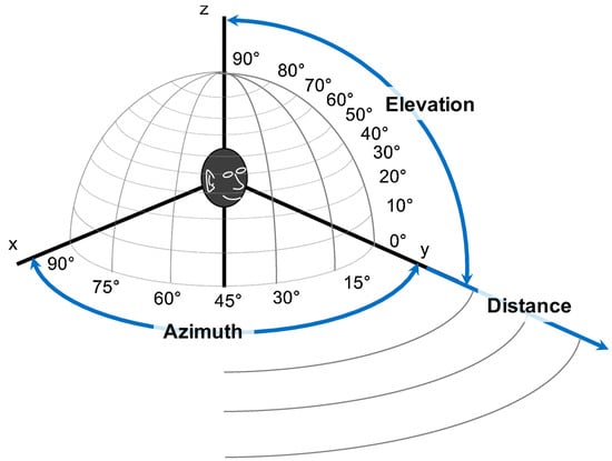
Figure 1. Polar coordinates ^[22].

This is due to the need to quickly update the estimated localization of the sound source ^[23]. In addition, the physical phenomena occurring during sound propagation in an elastic medium are of great importance. Sound reflected from several boundary surfaces, with the direct sound from the source and sounds from other localizations, can build up such a complex sound field that even the most accurate analysis cannot fully describe it ^[24]. These challenges make the subject of acoustic detection and localization a complex issue, the solution of which requires complex computational algorithms.

2. Acoustic Source Detection and Localization Methods

2.1. Classic Methods

Classic methods have stood the test of time and are still widely used due to their simplicity, reliability, and effectiveness. There are three main mathematical methods for determining the sound source. These include triangulation, trilateration, and multilateration ^[25]. They are described below:

Triangulation—Employs the geometric characteristics of triangles for localization determination. This approach calculates the angles at which acoustic signals arrive at the microphones. To establish a two-dimensional localization, a minimum of two microphones is requisite. For precise spatial coordinates, a minimum of three microphones is indispensable. It is worth noting that increasing the number of microphones amplifies the method’s accuracy. Moreover, the choice of microphone significantly influences the precision of the triangulation. Employing directional microphones enhances the accuracy by precisely capturing the directional characteristics of sound. Researchers in ^[26] demonstrated the enhanced outcomes of employing four microphones in a relevant study. The triangulation schema is shown on Figure 2.
Trilateration—Used to determine localization based on the distance to three microphones (Figure 3). Each microphone captures the acoustic signal at a different time, based on which the distance to the sound source is calculated. On this basis, the localization is determined by creating three circles with a radius corresponding to the distances from the microphones. The intersection point is the localization of the sound source ^[27]. It is less dependent on the directional characteristics of the microphones, potentially providing more flexibility in microphone selection.
Multilateration—Used to determine the localization based on four or more microphones. The principle of operation is identical to trilateration. Using more reference points allows for a more accurate determination of the localization because, with their help, measurement errors can be compensated. However, this results in greater complexity and computational requirements. Despite this increased intricacy, the accuracy and error mitigation benefits make multilateration a crucial technique in applications where precise localization determination is paramount ^[28].

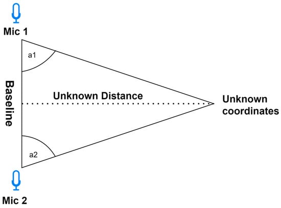
Figure 2. Two-dimensional triangulation schema.

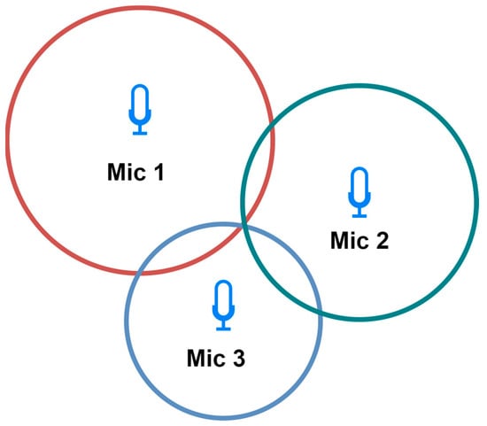
Figure 3. Two-dimensional trilateration schema.

To ascertain localizations using the above-mentioned methods, it is necessary to establish the parameters the method implies. The most popular are Time of Arrival (ToA), Time Difference of Arrival (TDoA), Time of Flight (ToF), and Angle of Arrival (AoA), often referred to as Direction of Arrival (DoA) ^[29]. They are described below:

Time of Arrival—This method measures the time from when the source emits the sound until the microphones detect the acoustic signal. Based on these data, it is possible to calculate the time it takes for the signal to reach the microphone. In ToA measurements, it is a requirement that the sensors and the source cooperate with each other, e.g., by synchronizing the time between them. The use of more microphones increases the accuracy of the measurements. This is due to the larger amount of data to be processed ^[30].
Time Difference of Arrival—This method measures the difference in time taken to capture the acoustic signal by microphones placed in different localizations. This makes it possible to determine the distance to a sound source based on the difference in the arrival times of the signals at the microphones based on the speed of sound in a given medium. The use of the TDoA technique requires information about the localization of the microphones and their acoustic characteristics, which include sensitivity and directionality. With these data, it is possible to determine the localization of the sound source using computational algorithms. For this purpose, the Generalized Cross-Correlation Function (GCC) is most often used ^[31]. Localizing a moving sound source using the TDoA method is a problem due to the Doppler effect ^[32].
Angle of Arrival—This method determines the angle at which the sound wave reaches the microphone. There are different ways to determine the angles. These include time-delay estimation, the MUSIC algorithm ^[33], and the ESPRIT algorithm ^[34]. Additionally, the sound wave frequency in spectral analysis can be used to estimate the DoA. As in the ToA, the accuracy of this method depends on the number of microphones, but the coherence of the signals is also very important. Since each node conducts individual estimations, synchronization is unnecessary ^[35].
Received Signal Strength—This method measures the intensity of the received acoustic signal and compares it with the signal attenuation model in a given medium. This is difficult to achieve due to multipath and shadow fading ^[36]. However, compared to Time of Arrival, it does not require time synchronization, and is not affected by the clock skew and clock offset ^[37].
Frequency Difference of Arrival (FDoA)—This method measures the frequency difference of the sound signal between two or more microphones ^[38]. Unlike TDoA, FDoA requires relative motion between observation points and the sound source, leading to varying Doppler shifts at different observation localizations due to the source’s movement. Sound source localization accuracy using FDoA depends on the signal bandwidth, signal-to-noise ratio, and the geometry of the sound source and observation points.
Time of Flight—This method measures the time from when the source emits the sound until the microphone detects the acoustic signal, including the additional time needed for the receiver to process the signal. Therefore, the duration is longer than in ToA ^[39]^[40].
Beamforming—Beamforming is an acoustic imaging technique that uses the power of microphone arrays to capture sound waves originating from various localizations. This method processes the collected audio data to generate a focused beam that concentrates sound energy in a specified direction. By doing so, it effectively pinpoints the source of sound within the environment. This is achieved by estimating the direction of incoming sound signals and enhancing them from desired angles, while suppressing noise and interference from other directions. Beamforming stands out as a robust solution, particularly when dealing with challenges such as reverberation and disturbances. However, it is important to note that in cases involving extensive microphone arrays, the computational demands can be relatively high ^[41]. An additional challenge posed by these methods is the localization of sources at low frequencies and in environments featuring partially or fully reflecting surfaces. In such scenarios, conventional beamforming techniques may fail to yield physically reasonable source maps. Moreover, the presence of obstacles introduces a further complication, as they cannot be adequately considered in the source localization process ^[42].
Energy-based—This technique uses the energy measurements gathered by sensors in a given area. By analyzing the energy patterns detected at different sensor localizations, the method calculates the likely localizations of the sources, taking into account factors such as noise and the decay of acoustic energy over distance. Compared to other methods, such as TDoA and DoA, energy-based techniques require a low sampling rate, leading to reduced communication costs. Additionally, these methods do not require time synchronization, often yielding lower precision compared to alternative methods ^[43].

The methods mentioned above have been used many times in practical solutions and described in the literature: ToA ^[44]^[45]^[46]^[47], TDoA ^[48]^[49], AoA ^[50], and RSS ^[51]. The most popular are Time Difference of Arrival and Angle of Arrival. The authors of ^[52] claim that the fusion of measurement data obtained using different measurement techniques can improve the accuracy. This is due to the inherent limitations of each localization estimation technique. An example of such an application is TDoA with AoA ^[38] or ToF with AoA ^[53].

In addition to the methods mentioned above, there are also signal-processing methods used in order to estimate the parameters of the above-mentioned methods. The most popular are described below:

Delay-and-Sum (DAS)—The simplest and the most popular beamforming algorithm. The principle of this algorithm is based on delaying the received signals at every microphone in order to compensate the signals’ relative arrival time delays. The algorithms generate an array of beamforming signals by processing the acoustic signals. These signals are combined to produce a consolidated beam that amplifies the desired sound while suppressing noise originating from other directions ^[41]^[54]. This method has a drawback of yielding poor spatial resolution, which leads to so-called ghost images, meaning that the beamforming algorithm outputs additional, non-existing sources. However, this problem can be addressed by using deconvolution beamforming and implementing the Point Spread Function, which is based on increasing the spatial resolution by examining the beamformer’s output at specific points ^[55]. The basic idea is shown in Figure 4.
Minimum Variance Distortion-less Response (MVDR)—A beamforming-based algorithm that introduces a compromise between reverberation and background noise. It evaluates the power of the received signal in all possible directions. MVDR sets the beamformer gain to be 1 in the direction of the desired signal, effectively enhancing its reception. This step allows the algorithm to focus on the primary signal of interest. By dynamically optimizing beamforming coefficients, MVDR enhances the discernibility of target signals while diminishing unwanted acoustic components. It provides higher resolution than DAM and LMS methods ^[56].
Multiple Signal Classifier (MUSIC)—The fundamental concept involves performing characteristic decomposition on the covariance matrix of any array output data, leading to the creation of a signal subspace that is orthogonal to a noise subspace associated with the signal components. Subsequently, these two distinct subspaces are employed to form a spectral function, obtained through spectral peak identification, enabling the detection of DoA signals. This algorithm exhibits high resolution, precision, and consistency when the precise arrangement and calibration of the microphone array are well established. In contrast, ESPRIT is more resilient and does not require searching for all potential directions of arrival, which results in lower computational demands ^[33].
Estimation of Signal Parameters via Rotational Invariance Techniques (ESPRIT)—This technique was initially developed for frequency estimation, but it has found a significant application in DoA estimation. ESPRIT is similar to the MUSIC algorithm in that it capitalizes on the inherent models of signals and noise, providing estimates that are both precise and computationally efficient. This technique leverages a property called shift invariance, which helps mitigate the challenges related to storage and computational demands. Importantly, ESPRIT does not necessitate precise knowledge of the array manifold steering vectors, eliminating the need for array calibration ^[57].
Steered Response Power (SRP)—This algorithm is widely used for beamforming-based localization. It estimates the direction of a sound source using the spatial properties of signals received by a microphone array. The SRP algorithm calculates the power across different steering directions and identifies the direction associated with the maximum power ^[58]. SRP is often combined with Phase Transform (PHAT) filtration to broaden the signal spectrum to improve the spatial resolution of SRP ^[59] and features robustness against nose and reverberation. However, it has disadvantages, such as heavy computation due to the grid search scheme, which limits its real-time usage ^[60].
Generalized Cross-Correlation—One of the most widely used cross-correlation algorithms. It operates by determining the phase using time disparities, acquiring the correlation function featuring a sharp peak, identifying the moment of highest correlation, and then merging this with the sampling rate to derive directional data ^[61].

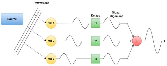
Figure 4. Delay and sum basic idea.

Each method mentioned above has distinct prerequisites, synchronization challenges, benefits, and limitations. The choice of which method to employ depends on the specific usage scenario, the balance between the desired accuracy, and the challenges posed by the environment in which the acoustic source localization is conducted.

The same principle applies for methods concerning sound source detection. Among them is the hidden Markov model (HMM). This model stands out as one of the most widely adopted classifiers for sound source detection. HMMs are characterized by a finite set of states, each representing a potential sound source class, and probabilistic transitions between these states to capture the dynamic nature of audio signals. In the context of sound source detection, standard features, such as Mel-Frequency Cepstral Coefficients (MFCC), are often employed in conjunction with HMMs. These features, such as MFCC, serve to extract relevant spectral characteristics from audio signals, providing a compact representation conducive to analysis by HMMs. During the training phase, HMMs learn the statistical properties associated with each sound source class, utilizing algorithms such as the Baum–Welch or Viterbi algorithm. The learning process allows HMMs to adapt to specific sound source classes and improve the detection accuracy over time. HMMs can be extended to model complex scenarios, such as multiple overlapping sound sources or varying background noise. However, HMMs are not without limitations. They assume stationarity, implying that the statistical properties of the signal remain constant over time, which may not hold true in rapidly changing sound environments. The finite memory of HMMs limits their ability to capture long-term dependencies in audio signals, particularly in dynamic acoustic scenes. Sensitivity to model parameters and the quality of training data pose challenges, and the computational complexity of the Viterbi decoding algorithm may be demanding for large state spaces ^[62].

2.2. Artificial Intelligence Methods

In recent years, there has been significant development of artificial intelligence. It has a wide range of applications, which results in its vast impact in many fields of science. Acoustic detection and localization is also such a field. Unlike methods focused on localization, which aim to directly determine the spatial coordinates of sound sources, AI-based detection methods often involve pattern matching and analysis of learned features to identify the presence or absence of specific sounds ^[63].

Convolutional Neural Networks (CNNs) are the most widely recognized deep learning models (Figure 5). CNN is a deep learning algorithm that can take an input image, assign weights to different objects in the image, and be able to distinguish one from another ^[64]. In ^[65], the authors proposed an approach based on the estimation of the DoA parameter. The phase components of the Short-Time Fourier Transform (STFT) coefficients of the received signals were adopted as input data, and the training consisted in learning the features needed for DoA estimation. This method turned out to be effective in adapting to unprecedented acoustic conditions. The authors proposed another interesting solution in ^[66]. They proposed the use of phase maps to estimate the DoA parameter. In CNN-based acoustic localization, a phase map visualizes the phase difference between two audio signals a pair of microphones picked up. By calculating the phase difference between the signals, it is possible to estimate the Direction of Arrival (DoA) of the sound source. The phase map is often used as an input feature for a CNN, allowing the network to learn to associate certain phase patterns with the direction of the sound source.

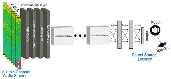
Figure 5. Example of CNN architecture ^[67].

An additional network architecture to consider is the Residual Neural Network, commonly known as ResNet. It was first introduced in ^[68]. It was designed in such a way that it avoids the phenomenon of the vanishing gradient. This makes it harder for the first layers of the model to learn essential features from the input data, leading to slower convergence or even stagnation in training ^[69]. As seen in the literature, the authors have proposed many solutions with ResNet networks in recent years. In ^[70], the authors proposed an approach to sound source localization using a single microphone. The network was trained on simulated data from a geometric sound propagation model in a given environment. In turn, the authors of ^[71] proposed a solution using ResNet and CNN (ResCNN). The authors used Squeeze-Excitation (SE) blocks to recalibrate feature maps. The modules were designed to improve the modeling of interdependencies between input feature channels compared to classic convolutional layers. Additionally, a noteworthy example of utilizing the ResNet architecture was presented in ^[72]. This solution combines Residual Networks with a channel attention module to enhance the efficiency of time–frequency information utilization. The residual network extracts input features, which are then weighted using the attention module. This novel approach demonstrates remarkable results when compared to popular baseline architectures based on Convolutional Recurrent Neural Networks and other improved models. It outperforms them in terms of localization accuracy and error, achieving an impressive average accuracy of nearly 98%.

In the context of sound source localization, transformers offer a unique and effective approach. They excel in processing sequences of data, making them well suited for tasks that involve analyzing audio signals over time. By leveraging their self-attention mechanisms and deep neural networks, transformers can accurately pinpoint the origin of sound sources within an environment. In ^[73], the author introduced a novel model, called the Binaural Audio Spectrogram Transformer (BAST), for sound azimuth prediction in both anechoic and reverberant environments. The author’s approach was employed to surpass CNN-based models, as CNNs exhibited limitations in capturing global acoustic features. The Transformer model, with its attention mechanism, overcomes this limitation. In this solution, the author has used three transformer encoders. The model is shown in Figure 6.

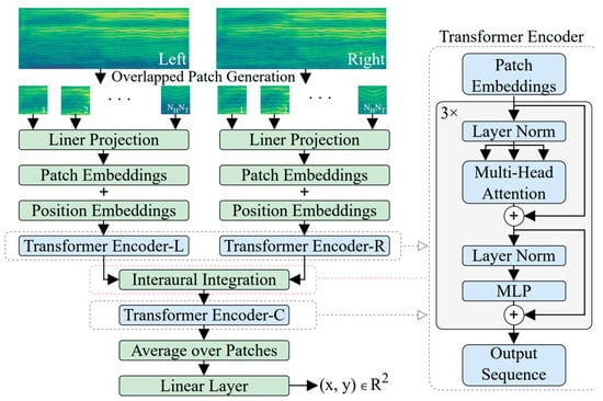
Figure 6. Attention-based model ^[73].

A dual-input hierarchical architecture is utilized to simulate the human subcortical auditory pathway. The spectrogram is initially divided into overlapping patches, which help capture more context from input data. Each patch undergoes a linear projection to transform its features to learn appropriate representations for each patch. The resulting linearly projected patches are then embedded into a vector space, and position embeddings are added to capture temporal relationships of the spectrogram in the Transformer. These embeddings are fed into a transformer encoder, which employs multi-head attention to capture both local and global dependencies within the spectrogram data. Following the transformer encoder, there is an interaural integration step, where two instances of the aforementioned architecture process the left and right channel spectrograms independently. The outputs from the two channels are integrated and fed into another transformer encoder to process the features together to produce the final results as sound localization coordinates.

An encoder–decoder network comprises two key components: an encoder that takes input features and produces a distinct representation of the input data, and a decoder that converts this encoded data into the desired output information. This architectural concept has been extensively studied in the field of deep learning and finds applications in various domains, including sound source localization. The authors of ^[74] proposed a method based on Autoencoders (AE). In their method, they employed a group of AEs, with each AE dedicated to reproducing the input signal from a specific candidate source localization within a multichannel environment. As each channel contains common latent information, representing the signal, individual encoders effectively separate the signal from their respective microphones. If the source indeed resides at the assumed localization, these estimated signals should closely resemble each other. Consequently, the localization process relies on identifying the AE with the most consistent latent representation.

Within the realm of literature, one can discover hybrid neural network approaches that seamlessly integrate both sound and visual representations. These approaches frequently involve the utilization of two distinct networks, each tailored to handle specific modalities. One network is typically dedicated to processing audio data, while the other specializes in visual information. One of those methods is proposed in ^[75] and is named SSLNet. The input data are a pair of sound and image. The sound signal is a 1D raw waveform and the image is a single frame taken from the video. Then, both are processed to a 2D spectrogram before they are fed to the neural networks.

References

Akhtar, N.; Saddique, M.; Asghar, K.; Bajwa, U.I.; Hussain, M.; Habib, Z. Digital Video Tampering Detection and Localization: Review, Representations, Challenges and Algorithm. Mathematics 2022, 10, 168.
Widodo, S.; Shiigi, T.; Hayashi, N.; Kikuchi, H.; Yanagida, K.; Nakatsuchi, Y.; Ogawa, Y.; Kondo, N. Moving Object Localization Using Sound-Based Positioning System with Doppler Shift Compensation. Robotics 2013, 2, 36–53.
Olesiński, A.; Piotrowski, Z. An Adaptive Energy Saving Algorithm for an RSSI-Based Localization System in Mobile Radio Sensors. Sensors 2021, 21, 3987.
Pontillo, V.; d’Aragona, D.A.; Pecorelli, F.; Di Nucci, D.; Ferrucci, F.; Palomba, F. Machine Learning-Based Test Smell Detection. arXiv 2022, arXiv:2208.07574.
Danilovich, S.; Shalev, G.; Boonman, A.; Goldshtein, A.; Yovel, Y. Echolocating Bats Detect but Misperceive a Multidimensional Incongruent Acoustic Stimulus. Proc. Natl. Acad. Sci. USA 2020, 117, 28475–28484.
Vance, H.; Madsen, P.T.; Aguilar De Soto, N.; Wisniewska, D.M.; Ladegaard, M.; Hooker, S.; Johnson, M. Echolocating Toothed Whales Use Ultra-Fast Echo-Kinetic Responses to Track Evasive Prey. eLife 2021, 10, e68825.
Nagesha, P.V.; Anand, G.V.; Kalyanasundaram, N.; Gurugopinath, S. Detection, Enumeration and Localization of Underwater Acoustic Sources. In Proceedings of the 2019 27th European Signal Processing Conference (EUSIPCO), A Coruna, Spain, 2–6 September 2019; IEEE: Piscataway, NJ, USA, 2019; pp. 1–5.
Kotus, J.; Lopatka, K.; Czyzewski, A. Detection and Localization of Selected Acoustic Events in Acoustic Field for Smart Surveillance Applications. Multimed. Tools Appl. 2014, 68, 5–21.
Argentieri, S.; Danès, P.; Souères, P. A Survey on Sound Source Localization in Robotics: From Binaural to Array Processing Methods. Comput. Speech Lang. 2015, 34, 87–112.
Rascon, C.; Meza, I. Localization of Sound Sources in Robotics: A Review. Robot. Auton. Syst. 2017, 96, 184–210.
Basiri, M.; Schill, F.; Lima, P.U.; Floreano, D. Robust Acoustic Source Localization of Emergency Signals from Micro Air Vehicles. In Proceedings of the 2012 IEEE/RSJ International Conference on Intelligent Robots and Systems, Vilamoura-Algarve, Portugal, 7–12 October 2012; IEEE: Piscataway, NJ, USA, 2012; pp. 4737–4742.
Khanal, A.; Chand, D.; Chaudhary, P.; Timilsina, S.; Panday, S.P.; Shakya, A. Search Disaster Victims Using Sound Source Localization. arXiv 2020, arXiv:2103.06049.
Nsalo Kong, D.F.; Shen, C.; Tian, C.; Zhang, K. A New Low-Cost Acoustic Beamforming Architecture for Real-Time Marine Sensing: Evaluation and Design. JMSE 2021, 9, 868.
Hożyń, S. A Review of Underwater Mine Detection and Classification in Sonar Imagery. Electronics 2021, 10, 2943.
Belloch, J.A.; Badia, J.M.; Igual, F.D.; Cobos, M. Practical Considerations for Acoustic Source Localization in the IoT Era: Platforms, Energy Efficiency, and Performance. IEEE Internet Things J. 2019, 6, 5068–5079.
Sanchez-Matilla, R.; Wang, L.; Cavallaro, A. Multi-Modal Localization and Enhancement of Multiple Sound Sources from a Micro Aerial Vehicle. In Proceedings of the Proceedings of the 25th ACM international conference on Multimedia, Mountain View, CA, USA, 23–27 October 2017; ACM: New York, NY, USA, 2017; pp. 1591–1599.
Wu, X.; Wu, Z.; Ju, L.; Wang, S. Binaural Audio-Visual Localization. Proc. AAAI Conf. Artif. Intell. 2021, 35, 2961–2968.
Manamperi, W.; Abhayapala, T.D.; Zhang, J.; Samarasinghe, P.N. Drone Audition: Sound Source Localization Using On-Board Microphones. IEEE/ACM Trans. Audio Speech Lang. Process. 2022, 30, 508–519.
Odya, P.; Kotus, J.; Kurowski, A.; Kostek, B. Acoustic Sensing Analytics Applied to Speech in Reverberation Conditions. Sensors 2021, 21, 6320.
Moragues, J.; Vergara, L.; Gosalbez, J.; Machmer, T.; Swerdlow, A.; Kroschel, K. Background Noise Suppression for Acoustic Localization by Means of an Adaptive Energy Detection Approach. In Proceedings of the 2008 IEEE International Conference on Acoustics, Speech and Signal Processing, Las Vegas, NV, USA, 31 March–4 April 2008; IEEE: Piscataway, NJ, USA, 2008; pp. 2421–2424.
Ouyang, K.; Xiong, W.; He, Q.; Peng, Z. Doppler Distortion Removal in Wayside Circular Microphone Array Signals. IEEE Trans. Instrum. Meas. 2019, 68, 1238–1251.
Risoud, M.; Hanson, J.-N.; Gauvrit, F.; Renard, C.; Lemesre, P.-E.; Bonne, N.-X.; Vincent, C. Sound Source Localization. Eur. Ann. Otorhinolaryngol. Head. Neck Dis. 2018, 135, 259–264.
Evers, C.; Loellmann, H.; Mellmann, H.; Schmidt, A.; Barfuss, H.; Naylor, P.; Kellermann, W. The LOCATA Challenge: Acoustic Source Localization and Tracking. IEEE/ACM Trans. Audio Speech Lang. Process. 2020, 28, 1620–1643.
Weyna, S. Identification of reflection, diffraction and scattering effects in real acoustic flow fields. Arch. Acoust. 2003, 28, 191–203.
Mahapatra, C.; Mohanty, A.R. Explosive Sound Source Localization in Indoor and Outdoor Environments Using Modified Levenberg Marquardt Algorithm. Measurement 2022, 187, 110362.
Lee, S.Y.; Chang, J.; Lee, S. Deep Learning-Enabled High-Resolution and Fast Sound Source Localization in Spherical Microphone Array System. IEEE Trans. Instrum. Meas. 2022, 71, 3161693.
Costa-Felix, R.; Machado, J.C.; Alvarenga, A.V. (Eds.) XXVI Brazilian Congress on Biomedical Engineering: CBEB 2018, Armação de Buzios, RJ, Brazil, 21–25 October 2018 (Vol. 1); IFMBE Proceedings; Springer: Singapore, 2019; Volume 70/1, ISBN 9789811321184.
Kapoor, R.; Ramasamy, S.; Gardi, A.; Bieber, C.; Silverberg, L.; Sabatini, R. A Novel 3D Multilateration Sensor Using Distributed Ultrasonic Beacons for Indoor Navigation. Sensors 2016, 16, 1637.
Ravindra, S.; Jagadeesha, S.N. Time of Arrival Based Localization in Wireless Sensor Networks: A Linear Approach. Signal Image Process. Int. J. 2013, 4, 13–30.
O’Keefe, B. Finding Location with Time of Arrival and Time Difference of Arrival Techniques. ECE Sr. Capstone Proj. 2017. Available online: https://sites.tufts.edu/eeseniordesignhandbook/files/2017/05/FireBrick_OKeefe_F1.pdf (accessed on 3 November 2023).
Knapp, C.; Carter, G. The Generalized Correlation Method for Estimation of Time Delay. IEEE Trans. Acoust. Speech Signal Process. 1976, 24, 320–327.
Hosseini, M.S.; Rezaie, A.; Zanjireh, Y. Time Difference of Arrival Estimation of Sound Source Using Cross Correlation and Modified Maximum Likelihood Weighting Function. Sci. Iran. 2017, 24, 3268–3279.
Tang, H.; Nordebo, S.; Cijvat, P. DOA Estimation Based on MUSIC Algorithm. 2014. Available online: https://www.diva-portal.org/smash/record.jsf?pid=diva2%3A724272&dswid=2353 (accessed on 3 November 2023).
Ning, Y.-M.; Ma, S.; Meng, F.-Y.; Wu, Q. DOA Estimation Based on ESPRIT Algorithm Method for Frequency Scanning LWA. IEEE Commun. Lett. 2020, 24, 1441–1445.
Dhabale, A. Direction Of Arrival (DOA) Estimation Using Array Signal Processing. Master’s Thesis, UC Riverside, Riverside, CA, USA, 2018.
Tan, H.-P.; Diamant, R.; Seah, W.K.G.; Waldmeyer, M. A Survey of Techniques and Challenges in Underwater Localization. Ocean. Eng. 2011, 38, 1663–1676.
Zhang, B.; Wang, H.; Xu, T.; Zheng, L.; Yang, Q. Received Signal Strength-Based Underwater Acoustic Localization Considering Stratification Effect. In Proceedings of the OCEANS 2016, Shanghai, China, 10–13 April 2016; IEEE: Piscataway, NJ, USA, 2016; pp. 1–8.
Kraljevic, L.; Russo, M.; Stella, M.; Sikora, M. Free-Field TDOA-AOA Sound Source Localization Using Three Soundfield Microphones. IEEE Access 2020, 8, 87749–87761.
Pinheiro, B.C.; Moreno, U.F.; De Sousa, J.T.B.; Rodriguezz, O.C. Improvements in the Estimated Time of Flight of Acoustic Signals for AUV Localization. In Proceedings of the 2013 MTS/IEEE OCEANS, Bergen, NJ, USA, 10–14 June 2013; IEEE: Piscataway, NJ, USA, 2013; pp. 1–6.
De Marziani, C.; Urena, J.; Hernandez, Á.; Garcia, J.J.; Alvarez, F.J.; Jimenez, A.; Perez, M.C.; Carrizo, J.M.V.; Aparicio, J.; Alcoleas, R. Simultaneous Round-Trip Time-of-Flight Measurements With Encoded Acoustic Signals. IEEE Sens. J. 2012, 12, 2931–2940.
Chiariotti, P.; Martarelli, M.; Castellini, P. Acoustic Beamforming for Noise Source Localization—Reviews, Methodology and Applications. Mech. Syst. Signal Process. 2019, 120, 422–448.
Gombots, S.; Nowak, J.; Kaltenbacher, M. Sound Source Localization—State of the Art and New Inverse Scheme. Elektrotech. Inftech. 2021, 138, 229–243.
Energy Based Acoustic Source Localization|SpringerLink. Available online: https://link.springer.com/chapter/10.1007/3-540-36978-3_19 (accessed on 3 November 2023).
Diamant, R.; Kastner, R.; Zorzi, M. Detection and Time-of-Arrival Estimation of Underwater Acoustic Signals. In Proceedings of the 2016 IEEE 17th International Workshop on Signal Processing Advances in Wireless Communications (SPAWC), Edinburgh, UK, 3–6 July 2016; IEEE: Piscataway, NJ, USA, 2016; pp. 1–5.
Diamant, R. Clustering Approach for Detection and Time of Arrival Estimation of Hydrocoustic Signals. IEEE Sens. J. 2016, 16, 5308–5318.
Zou, Y.; Liu, H. A Simple and Efficient Iterative Method for Toa Localization. In Proceedings of the ICASSP 2020—2020 IEEE International Conference on Acoustics, Speech and Signal Processing (ICASSP), Barcelona, Spain, 4–8 May 2020; IEEE: Piscataway, NJ, USA, 2020; pp. 4881–4884.
Zhang, L.; Chen, M.; Wang, X.; Wang, Z. TOA Estimation of Chirp Signal in Dense Multipath Environment for Low-Cost Acoustic Ranging. IEEE Trans. Instrum. Meas. 2019, 68, 355–367.
Khyzhniak, M.; Malanowski, M. Localization of an Acoustic Emission Source Based on Time Difference of Arrival. In Proceedings of the 2021 Signal Processing Symposium (SPSympo), Lodz, Poland, 20–23 September 2021; IEEE: Piscataway, NJ, USA, 2021; pp. 117–121.
Dang, X.; Ma, W.; Habets, E.A.P.; Zhu, H. TDOA-Based Robust Sound Source Localization With Sparse Regularization in Wireless Acoustic Sensor Networks. IEEE/ACM Trans. Audio Speech Lang. Process. 2022, 30, 1108–1123.
Astapov, S.; Berdnikova, J.; Ehala, J.; Kaugerand, J.; Preden, J.-S. Gunshot Acoustic Event Identification and Shooter Localization in a WSN of Asynchronous Multichannel Acoustic Ground Sensors. Multidim Syst. Sign Process 2018, 29, 563–595.
Poursheikhali, S.; Zamiri-Jafarian, H. Source Localization in Inhomogeneous Underwater Medium Using Sensor Arrays: Received Signal Strength Approach. Signal Process. 2021, 183, 108047.
De Gante, A.; Siller, M. A Survey of Hybrid Schemes for Location Estimation in Wireless Sensor Networks. Procedia Technol. 2013, 7, 377–383.
Van Kleunen, W.A.P.; Blom, K.C.H.; Meratnia, N.; Kokkeler, A.B.J.; Havinga, P.J.M.; Smit, G.J.M. Underwater Localization by Combining Time-of-Flight and Direction-of-Arrival. In Proceedings of the OCEANS 2014, Taipei, Taiwan, 7–10 April 2014; IEEE: Piscataway, NJ, USA, 2014; pp. 1–6.
Hassan, F.; Mahmood, A.K.B.; Yahya, N.; Saboor, A.; Abbas, M.Z.; Khan, Z.; Rimsan, M. State-of-the-Art Review on the Acoustic Emission Source Localization Techniques. IEEE Access 2021, 9, 101246–101266.
Lee, S.Y.; Chang, J.; Lee, S. Deep Learning-Based Method for Multiple Sound Source Localization with High Resolution and Accuracy. Mech. Syst. Signal Process. 2021, 161, 107959.
Cohen, I.; Benesty, J.; Gannot, S. (Eds.) Speech Processing in Modern Communication: Challenges and Perspectives; Springer Topics in Signal Processing; Springer: Berlin/Heidelberg, Germany, 2010; Volume 3, ISBN 978-3-642-11129-7.
Kasthuri, N.; Balambigai, S.; Yuvashree, S. Source Localization for Underwater Acoustics Using Esprit Algorithm. IOP Conf. Ser. Mater. Sci. Eng. 2021, 1055, 012023.
Traa, J.; Wingate, D.; Stein, N.D.; Smaragdis, P. Robust Source Localization and Enhancement With a Probabilistic Steered Response Power Model. IEEE/ACM Trans. Audio Speech Lang. Process. 2016, 24, 493–503.
Salvati, D.; Drioli, C.; Foresti, G.L. Acoustic Source Localization Using a Geometrically Sampled Grid SRP-PHAT Algorithm With Max-Pooling Operation. IEEE Signal Process. Lett. 2022, 29, 1828–1832.
Zhuo, D.-B.; Cao, H. Fast Sound Source Localization Based on SRP-PHAT Using Density Peaks Clustering. Appl. Sci. 2021, 11, 445.
Saxena, A.; Ng, A.Y. Learning Sound Location from a Single Microphone. In Proceedings of the 2009 IEEE International Conference on Robotics and Automation, Kobe, Japan, 12–17 May 2009; IEEE: Piscataway, NJ, USA, 2009; pp. 1737–1742.
Mesaros, A.; Heittola, T.; Eronen, A.; Virtanen, T. Acoustic event detection in real life recordings. In Proceedings of the 2010 18th European Signal Processing Conference, Aalborg, Denmark, 23–27 August 2010.
Vera-Diaz, J.M.; Pizarro, D.; Macias-Guarasa, J. Towards End-to-End Acoustic Localization Using Deep Learning: From Audio Signal to Source Position Coordinates. Sensors 2018, 18, 3418.
Yamashita, R.; Nishio, M.; Do, R.K.G.; Togashi, K. Convolutional Neural Networks: An Overview and Application in Radiology. Insights Imaging 2018, 9, 611–629.
Chakrabarty, S.; Habets, E.A.P. Multi-Speaker DOA Estimation Using Deep Convolutional Networks Trained With Noise Signals. IEEE J. Sel. Top. Signal Process. 2019, 13, 8–21.
Chakrabarty, S.; Habets, E.A.P. Broadband DOA Estimation Using Convolutional Neural Networks Trained with Noise Signals. In Proceedings of the 2017 IEEE Workshop on Applications of Signal Processing to Audio and Acoustics (WASPAA), New Paltz, NY, USA, 15–18 October 2017; IEEE: Piscataway, NJ, USA, 2017; pp. 136–140.
Yalta, N.; Nakadai, K.; Ogata, T.; Intermedia Art and Science Department, Waseda University; Honda Research Institute Japan Co., Ltd. Sound Source Localization Using Deep Learning Models. J. Robot. Mechatron. 2017, 29, 37–48.
He, K.; Zhang, X.; Ren, S.; Sun, J. Deep Residual Learning for Image Recognition. In Proceedings of the IEEE Computer Society Conference on Computer Vision and Pattern Recognition (CVPR), Las Vegas, NV, USA, 27–30 June 2016.
Residual Neural Network (ResNet). Available online: https://iq.opengenus.org/residual-neural-networks/ (accessed on 3 November 2023).
Kujawski, A.; Herold, G.; Sarradj, E. A Deep Learning Method for Grid-Free Localization and Quantification of Sound Sources. J. Acoust. Soc. Am. 2019, 146, EL225–EL231.
Naranjo-Alcazar, J.; Perez-Castanos, S.; Ferrandis, J.; Zuccarello, P.; Cobos, M. Sound Event Localization and Detection Using Squeeze-Excitation Residual CNNs. arXiv 2021, arXiv:2006.14436v3.
Hu, F.; Song, X.; He, R.; Yu, Y. Sound Source Localization Based on Residual Network and Channel Attention Module. Sci. Rep. 2023, 13, 5443.
Kuang, S.; van der Heijden, K.; Mehrkanoon, S. BAST: Binaural Audio Spectrogram Transformer for Binaural Sound Localization. arXiv 2022, arXiv:2207.03927v1.
Huang, Y.; Wu, X.; Qu, T. A Time-Domain Unsupervised Learning Based Sound Source Localization Method. In Proceedings of the 2020 IEEE 3rd International Conference on Information Communication and Signal Processing (ICICSP), Shanghai, China, 12–15 September 2020; IEEE: Piscataway, NJ, USA, 2020; pp. 26–32.
Feng, F.; Ming, Y.; Hu, N. SSLNet: A Network for Cross-Modal Sound Source Localization in Visual Scenes. Neurocomputing 2022, 500, 1052–1062.

© Text is available under the terms and conditions of the Creative Commons Attribution (CC BY) license; additional terms may apply. By using this site, you agree to the Terms and Conditions and Privacy Policy.

Upload a video for this entry

Information

Subjects: Mathematics

Contributors MDPI registered users' name will be linked to their SciProfiles pages. To register with us, please refer to https://encyclopedia.pub/register :

Gabriel Jekateryńczuk

Zbigniew Piotrowski

View Times: 199

Update Date: 28 Dec 2023

Table of Contents

Video Upload Options

Confirm