New Ways to Modelling and Predicting Ionosphere Variables

Version	Summary	Created by	Modification	Content Size	Created at	Operation
1		SANDRO RADICELLA	--	1860	2023-12-13 11:42:26	\|
2	Reference format revised.	Lindsay Dong	-2 word(s)	1858	2023-12-19 04:27:26	\|

This entry is adapted from the peer-reviewed paper 10.3390/atmos14121788

The new way of thinking science from Newtonian determinism to nonlinear unpredictability and the dawn of advanced computer science and technology can be summarized in the words of the theoretical physicist Michel Baranger, who, in 2000, said in a conference: “Twenty-first-century theoretical physics is coming out of the chaos revolution; it will be about complexity and its principal tool will be the computer.”. This can be extended to natural sciences in general. Modelling and predicting ionosphere variables have been considered since many decades as a paramount objective of research by scientists and engineers. The new approach to natural sciences influenced also ionosphere research. Ionosphere as a part of the solar–terrestrial environment is recognised to be a complex chaotic system, and its study under this new way of thinking should become an important area of ionospheric research, particularly with the addition of machine learning techniques.

ionosphere modelling complex systems

1. Introduction

1.1. About Linear and Complex Systems

In April 2000, the French-US theoretical physicist Michel Baranger gave a “physics talk for non-physicists” on chaos, complexity, and entropy at the New England Complex Systems Institute of Cambridge, Massachusetts ^[1]. In his initial words, he said, “Twentieth-century theoretical physics came out of the relativistic revolution and the quantum mechanical revolution. It was all about simplicity and continuity (in spite of quantum jumps). Its principal tool was calculus. Its final expression was field theory. Twenty-first century theoretical physics is coming out of the chaos revolution. It will be about complexity and its principal tool will be the computer. Its final expression remains to be found.”.

The “solar–terrestrial physics” phrase has been replaced in the last few decades by “space weather”. This was carried out to make the subject more appealing to the public and politicians and also to stress the effect of solar–terrestrial physics on technology. However, space weather should be considered just a part of solar–terrestrial physics, recognizing that it is the “star” of this field.

All physical sciences of the 20th century, including relativity and quantum mechanics, were based on “calculus” introduced by Newton and Leibnitz, by itself a key example of linear approach. Space and earth system sciences are data-driven, and they always had to rely on time series of observations of specific variables intrinsically not repeatable. Their time variations were analyzed, modelled, and forecasted on the basis of the model adopted. Models were grounded for a long time on linear approaches not only following Newton’s and Leibnitz’s “calculus” but also because of the reduced number of data available.

A linear system has a fixed proportional relationship between the input and output; it is predictable and stable. In addition, the relationship between variables x and y can be graphically represented by a straight line. The linear modelling efforts to explain the variability of data time series played an important role in understanding the basic behavior of natural phenomena. However, most natural processes are nonlinear, and, thus, linear models can only approximate real-world systems to a certain extent. A typical linear system approach is given by the Maxwell equations.

The advancement of experimental data sources, their increase in number, and particularly the advent of the space era and the enormous amount of space and ground data now available completely changed the perspective of solar–terrestrial physics/space weather.

1.2. About Complex Systems and Chaos

One of the characteristics of a complex system is its nonlinearity, and its modelling shows nonlinear relationships between inputs and outputs, as well as chaotic behavior often present in natural systems. When we say that a certain system “exhibits chaos”, it means that the system obeys deterministic time evolution, but that the outcome is highly sensitive to small uncertainties in the specification of the initial conditions, as indicated in the pioneering work of Lorenz (1963) ^[2].

A way to quantify the presence and degree of chaos in a complex system is to measure its correlation dimension (D₂) and the Kolmogorov entropy (K₂) (Abarbanel and Parlitz, 2006) ^[3], which can be calculated with the method given by Grassberger and Procaccia (1983a) ^[4].

The correlation dimension D₂ is a non-integer value and gives a lower limit of the number of independent variables or the degree of freedom of the system. It indicates the minimum number of differential equations needed to fully describe the system itself. A value of K₂ = 0 indicates a fully predictable evolution of the system, a finite K₂ > 0 indicates a chaotic system, and a value K₂ = ∞ indicates a fully stochastic system. An estimate of time predictability of a system variable is given by 1/K₂.

1.3. Solar–Terrestrial Physics/Space Weather and Chaos

Time series of observable variable data, processing of such data, modelling, and prediction are the essential steps of solar–terrestrial physics/space weather, including ionosphere research.

Let us assume that all the systems involved in the solar–terrestrial environment are complex. It is important to investigate if these complex systems exhibit chaotic behavior. This can be performed in terms of the correlation dimension and the Kolmogorov entropy mentioned above.

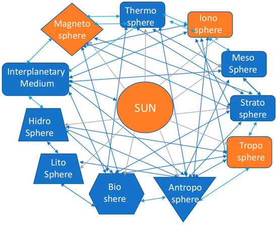
Considering that all the systems of the complex solar–terrestrial system are mutually interacting as indicated in Figure 1, those that are going to be analyzed in the discussion that follows are indicated in orange.

Figure 1. The assumed complex solar–terrestrial system of interacting complex systems (both blue and orange). In orange are those systems that are going to be considered in the text discussion. Light grey arrows indicate that the Sun act on all the other systems and blue arrows indicates that all the other systems may act among them.

2. An Overview of Ionosphere Variability

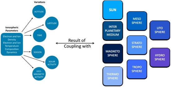
The multifaceted variability of the ionosphere due to the fact that it is a complex system interacting with complex systems is summarized in Figure 2.

Figure 2. Ionospheric variation result of interactions with other complex systems.

Following Mendillo (2020) ^[5] and the method developed by Rishbeth and Mendillo (2001) ^[6], three main sources of the day-to-day variability σ_total of NmF2 can be identified, where σ_total is the standard deviation of NmF2 daily values within every month. These are changes of ionizing photon solar radiation σ_sun, solar-wind-induced geomagnetic activity σ_mag, and meteorological coupling from the troposphere σ_met. The chosen groups of years can be written as

[σ_total]² = [σ_sun]² + [σ_mag]² + [σ_met]²

Under nominal conditions (in the absence of solar or geomagnetic events), Mendillo (2020) ^[5] considers that the total variability and contribution of each component of this variability in percentage (see the equation above) is

[20–25%]² = [3–6%]² + [14–17%]² + [14–17%]²

He concludes that the influence of ionizing photon solar radiation is minimal in comparison with solar wind magnetospheric sources and tropospheric sources, with the latter two being comparable. The same author considers that the results for NmF2 are also valid for the day-to-day variability of the TEC.

3. Chaos Theory and the Ionosphere

The analysis that follows will be centered on those studies that treat time series data of foF2 and TEC in terms of correlation dimension. Possible convergent or divergent results from different authors using diverse time series lengths and sampling rates will be evidenced in Table 1 and Table 2.

Table 1. Correlation dimension of the deterministic chaos found in foF2 time series by two different authors under different conditions. Geomagnetic activity not specified.

Latitude	Solar Activity (F10.7)	Geomagnetic Activity	foF2 Time Series Length	foF2 Sampling Rate	D	Authors
High	Low	---	2 years	1 h	3.4	Romanelli et al., 1988 ^[7]
Middle high	Low	---	83 days	1 h	3.0	Mendez, 2022 ^[8]
Middle high	Low	---	83 days	1 h	3.3	Mendez, 2022 ^[8]

Regarding foF2 data, I found only two papers analyzing the chaos characteristics of the time series. As shown in Table 1, the first study reporting the existence of a low dimension in an foF2 data series was the one of Romanelli et al. (1988). These authors used a time series of hourly values of foF2 obtained at Argentine Island (65.25° S, 64.27° W) for the years 1977–1978. A recent paper by Mendez (2022) ^[8] reports the study of chaos characteristics obtained from two foF2 time series obtained at Juliusruh (54.6° N 13.4° E) from 1 November 1987 to 10 February 1988 and from 1 November 2002 to 10 February 2003.

The large amount of TEC now available has allowed the study of the chaoticity of this ionosphere parameter by several authors.

Kumar et al. (2004) ^[9] reported the chaotic behavior of time series of TEC at a 15 min sampling rate at Goose Bay (47° N, 286° E) during the period February to April of the solar minimum year 1976. The TEC was measured by Faraday rotation technique using the trans-ionosphere signal from the satellite GOES-2.

These references were chosen because, in all of them, the correlation dimension is calculated. As indicated in the introduction, the correlation dimension is a good indicator of the type of chaoticity found in an experimental time series. Table 1 summarizes their results in terms of correlation dimension (D). It is organized by the latitude of the location considered and solar activity and by considering the geomagnetic activity also. The intention is to see if the results of different authors and calculation techniques, using the distinct length of the time series and data sampling rates, show a consistent picture.

Table 2. Correlation dimension of the deterministic chaos found in TEC time series by different authors under different conditions. The asterisk means that the values are the averages of those shown in Table 1 of the paper mentioned (Eapen et al., 2018). “---” indicate that the geomagnetic activity is not specified.

Latitude	Solar Activity (F10.7)	Geomagnetic Activity	TEC Time Series Length	TEC Sampling Rate	D	Authors
Low	Low	Quiet	4 days	1 min	2.23–2.74	Unnikrishnan (2010) ^[10]
Low	Low	Disturbed	4 days	1 min	3.37	Unnikrishnan (2010) ^[10]
Low	Low	Monthly 5 quiet days	1 year	1 min	3.5	Ogunsua (2013) ^[11]
Low	Low	Monthly 5 disturbed days	1 year	1 min	2.8	Ogunsua (2013) ^[11]
Low	Low	Quiet	4 months	5 min	4.61 *	Eapen et al. (2018) ^[12]
Low	Low	Disturbed	4 months	5 min	3.74 *	Eapen et al. (2018) ^[12]
Middle	Low	Quiet	4 months	5 min	4.63 *	Eapen et al. (2018) ^[12]
Middle	Low	Disturbed	4 months	5 min	3.81 *	Eapen et al. (2018) ^[12]
Middle	Low	---	1 year	1 min	2.78	Materassi et al. (2023) ^[13]
Middle	High	---	1 year	1 min	2.78	Materassi et al. (2023) ^[13]
High	Low	Two intense storms in the period	3 months (February–April)	15 min	5.63	Kumar et al. (2004) ^[9]
High	Low	Quiet	4 months	5 min	6.22 *	Eapen et al. (2018) ^[12]
High	Low	Disturbed	4 months	5 min	3.77 *	Eapen et al. (2018) ^[12]

Machine Learning and the Ionosphere

Machine learning (ML) has been increasingly applied to ionosphere time series data analysis in the past several decades to model and forecast their evolution. Research started by using artificial neural networks or, in brief, NNs. The first steps on NNs came in the 1940s, but it was in the 1980s when they evolved to what is now known about them. Between 2009 and 2012, the recurrent NNs and deep feedforward NNs were developed (Schmidhuber, 2014 ^[14]). Later on, NNs became the basis of what is known as deep learning (DL), a set or branch of ML. NNs are systems or hardware designed to operate in a way that imitates the work of human neurons. The simplest type of NNs is the feedforward NNs where the information moves in one direction, from the input nodes to the output nodes. The other main type of NNs is the recurrent NN that allows the output from some nodes to affect the subsequent input to the same nodes. Since the early 1990s, NNs of different type evolved to more advanced DL tools that have been used in ionosphere research with relevant success. They were performed to model and predict particularly the behavior of the TEC obtained from GNSS signals (most of them from the GPS constellation).

References

Baranger, M. Complexity, Chaos, and Entropy; New England Complex Systems Institute: Cambridge, MA, USA, 2000.
Lorenz, E.N. Deterministic nonperiodic flow. J. Atmos. Sci. 1963, 20, 130.
Abarbanel, H.D.I.; Parlitz, U. Nonlinear Analysis of Time Series Data. In Handbook of Time Series Analysis—Recent Theoretical Developments and Applications; Schelter, B., Winterhalder, M., Timmer, J., Eds.; John Wiley & Sons, Inc.: Hoboken, NJ, USA, 2006; ISBN 9783527406234.
Grassberger, P.; Procaccia, I. Characterization of Strange Attractors. Phys. Rev. Lett. 1983, 50, 346–349.
Mendillo, M. Day-to-day variability of the ionosphere. In The Dynamical Ionosphere; Elsevier: Amsterdam, The Netherlands, 2020; p. 442.
Rishbeth, H.; Mendillo, M. Patterns of F2-layer variability. J. Atmos. Sol. Terr. Phys. 2001, 63, 1661–1680.
Romanelli, L.; Figliola, M.A.; Hirsch, F.A. Deterministic chaos and natural phenomena. J. Stat. Phys. 1988, 53, 991–994.
Mendez, A.L. How deterministic is the Earth ionosphere’s response to solar activity? Astrophys. Space Sci. 2022, 367, 1–6.
Kumar, K.S.; Kumar, C.V.A.; George, B.; Renuka, G.; Venugopal, C. Analysis of the fluctuations of the total electron content (TEC) measured at Goose Bay using tools of nonlinear methods. J. Geophys. Res. Space Phys. 2004, 109, A02308.
Unnikrishnan, K. A comparative study on chaoticity of equatorial/low latitude ionosphere over Indian subcontinent during geomagnetically quiet and disturbed periods. Nonlinear Process. Geophys. 2010, 17, 765–776.
Ogunsua, B.O.; Laoye, J.A.; Fuwape, I.A.; Rabiu, A.B. The comparative study of chaoticity and dynamical complexity of the low-latitude ionosphere, over Nigeria, during quiet and disturbed days. Nonlinear Process. Geophys. 2014, 21, 127–142.
Eapen, S.; Asokan, K.; Kumar, K.S.; Ramamohan, T.R.; Kumar, A. Comparison of Variations of TEC at Disturbed and Quiet Time Using Nonlinear Dynamics Tools. J. Geophys. Res. Space Phys. 2018, 123, 7740–7754.
Materassi, M.; Alberti, T.; Migoya-Orué, Y.; Radicella, S.M.; Consolini, G. Chaos and Predictability in Ionospheric Time Series. Entropy 2023, 25, 368.
Schmidhuber, J. Deep Learning in Neural Networks: An Overview. Neural Netw. 2018, 61, 85–117.

© Text is available under the terms and conditions of the Creative Commons Attribution (CC BY) license; additional terms may apply. By using this site, you agree to the Terms and Conditions and Privacy Policy.

Upload a video for this entry

Information

Subjects: Meteorology & Atmospheric Sciences

Contributor MDPI registered users' name will be linked to their SciProfiles pages. To register with us, please refer to https://encyclopedia.pub/register :

Sandro M. Radicella

View Times: 109

Update Date: 19 Dec 2023

Table of Contents

Video Upload Options

Confirm