Hyperbolic Barriers in Geophysical Flows and Their Extraction

Version	Summary	Created by	Modification	Content Size	Created at	Operation
1		SERGEY PRANTS	--	1310	2023-10-23 09:24:11	\|
2	format correct	Catherine Yang	Meta information modification	1310	2023-10-23 10:09:32	\|

This entry is adapted from the peer-reviewed paper 10.3390/sym15101942

Transport barriers are material surfaces across which the transport is minimal. They can be classified into elliptic, parabolic, and hyperbolic barriers. Hyperbolic barriers are less evident. They are the most influential repelling and attracting material lines (or surfaces in 3D cases) with the strongest local stability, which can be identified in real oceanic and atmospheric flows by calculating the maximal Lyapunov exponents. The transport barriers are fundamental features controlling the movement of anthropogenic and natural pollutants, plankton, cross-shelf exchange, and the propagation of upwelling fronts in coastal zones.

elliptic parabolic hyperbolic transport barriers

1. Identification of Hyperbolic Barriers Using Lagrangian Coherent Structures

The elliptic and parabolic TBs are invariant manifolds associated with coherent features, like vortices and jets. The analysis of their destruction in simplified models was based on a temporal periodicity of perturbation. The majority of geophysical flows are not periodic in time. Nevertheless, hyperbolic points of a transient nature exist in quasi-turbulent flows, and their “effective” stable and unstable manifolds can be identified. Stable and unstable manifolds in steady and (quasi)-time-periodic flows are defined in the infinite time limit, whereas the effective manifolds in real geophysical flows “live” for a finite time. They partition a flow in dynamically and topologically distinct domains. In particular, the unstable effective manifolds are TBs, albeit temporary, which may separate water/air masses with different characteristics. Tracers cannot cross such barriers by purely advective processes, whereas there are strong gradients of tracers close to barriers with enhanced mixing in their vicinity.

The strict mathematical basis of using effective manifolds in aperiodic flows with the velocity defined for finite-time intervals was developed by G. Haller et al. ^[1]^[2]^[3], who introduced the concept of the so-called Lagrangian coherent structures (LCSs). Lagrangian coherent structures are defined as the material surfaces or curves that attract or repel particles at the highest local rate relative to other material surfaces nearby. Any flow is composed of a continuum of material surfaces, and the problem is to identify the surfaces with the strongest stability. Lagrangian coherent structures are those repelling and attracting structures that dominate in advection.

Lagrangian coherent structures consist of the same fluid elements, which is why they are Lagrangian. They exist longer and are more robust than adjacent material surfaces, which is why they are coherent. Figure 1 schematically illustrates how a blob with tracers, chosen near a repelling (stable) LCS, is advected toward the associated hyperbolic point over time. When approaching that point, the blob stretches along the attracting (unstable) manifold. The Lagrangian coherent structures are frame-invariant, whereas the unsteady velocity field may depend strongly on the reference frame.

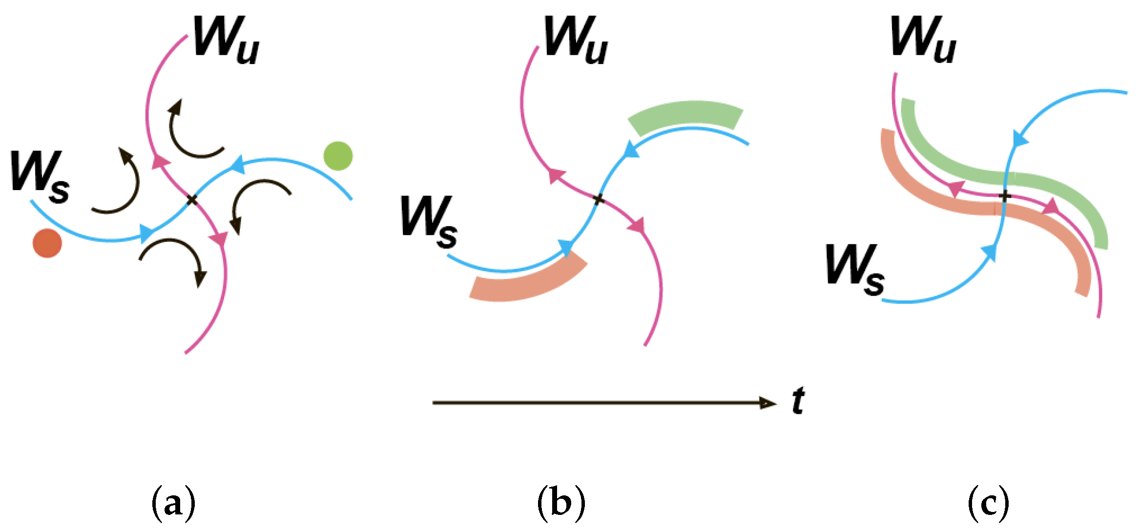
Figure 1. The illustration of an HTB near the associated hyperbolic point (cross). (a) The blobs with tracers approach this point along the repelling stable manifold

W_{s}

(b) and then are advected away from it along the attracting unstable manifold

W_{u}

. (c) The unstable manifold attracts all nearby fluid particles, stretches out the blobs to adopt its shape, and acts as an HTB for the tracers.

P. Pierrehumbert ^[4]^[5] introduced the computation of FTLE in geophysical velocity fields as a measure of chaotic mixing. G. Haller posited that, in 2D flows, ridges with locally maximal FTLE values approximate the locations of repelling and attracting LCSs in forward and backward time, respectively. These ridges can be operationally defined as local FTLE/FSLE extrema and have been proven to be almost Lagrangian with a small flux across them ^[1]^[2]^[3].

2. Some Remarks on the Simulation of Transport and Mixing Processes in Satellite-Derived Velocity Fields

The progress in satellite monitoring and development of high-resolution, eddy-resolving circulation models opened up new possibilities to study the transport and mixing in geophysical flows. A microwave satellite radar measures the distance to the ocean surface to obtain anomalies of the sea-surface level, allowing one to infer the velocity field in the geostrophic approximation where horizontal pressure gradients balance the Coriolis force. The resulting velocity field is altimetric. Daily geostrophic velocities, such as those from AVISO/CMEMS http://aviso.altimetry.fr are freely accessible from from 1 January 1993 to the present time. They are provided at a spatial resolution of, at minimum,

1 / 4^{\circ} \times 1 / 4^{\circ}

, and have a daily time step. These data are commonly used to calculate the advection of tracers in the ocean.

In the Lagrangian approach, advection equations are integrated for a substantial number of particles using either the altimetric velocity field or the velocity fields from circulation models and reanalyses provided on a discrete grid. Before solving these equations, numerical algorithms are necessary. In the 2D scenario, the equation takes a simple form:

where u and v are angular zonal and meridional velocities, which are convenient to use for solving advection equations on the Earth sphere,

ϕ

and

λ

are the latitude and longitude, respectively. The following procedure is commonly used ^[6]:

Bicubic interpolation of the velocity components in space, and time interpolation using third-order Lagrangian polynomials, conducted independently of each other.
Substituting the interpolated velocity values in Equation (1), which are integrated using the fourth order Runge–Kutta method.
Calculating the relevant Lagrangian indicators and representing their values on a geographic map of the study region.

Using the altimetric velocity field with relatively coarse resolution, the simulation results typically resolve mesoscale features. Moreover, this field is an approximation to the “real” velocity field in the ocean. It has been theoretically shown ^[1] that LCSs are robust to inevitable errors in velocity fields if LCSs are strong and exist for a sufficiently long time. Although simulated trajectories may diverge exponentially from “true” trajectories near a repelling LCS, the very LCSs are not expected to be perturbed to the same degree because numerical errors grow along the LCS. The FTLE/FSLE diagnostics in the altimetric velocity field are reliable at detecting mesoscale features and even smaller features if the latter ones evolve due to advection. The developing surface water and ocean topography (SWOT) mission provides the velocity field at much higher resolutions, down to a few kms, allowing to catch some submesoscale processes and features.

The Lagrangian simulation results are based not on individual trajectories but on hundreds of thousands and millions of trajectories. No one can guarantee that he/she is able to compute “true” chaotic trajectories of individual particles. The shadowing lemma in the theory of dynamical systems states that, roughly speaking, every numerically computed trajectory in strongly chaotic systems stays close to a “true” trajectory with a slightly altered initial position.

3. Lyapunov Exponents as Lagrangian Diagnostics

One of the commonly used Lagrangian diagnostics to quantify mixing in geophysical flows is a maximal Lyapunov exponent. The finite-time Lyapunov exponent can be calculated by different methods from advection equations. Following Ref. ^[7], FTLE in a 2D case is defined as follows:

where

σ_{1} (t, t_{0})

is the largest singular value of the evolution matrix, specifying how far away initially close particles diverge from each other over time, and

t - t_{0}

is the integration time.

The finite-scale Lyapunov exponent is calculated until the moment of time

τ

, when two particles, initially separated by a distance

δ_{0}

, diverge over a distance

δ_{f}

^[8]^[9]:

Both the diagnostics provide similar results.

To identify HTBs in geophysical flows, the spatial distributions of the FTLE (FSLE) values are computed forward and backward in time. A study area in the ocean or atmosphere is populated with a large number of artificial particles on a grid. The FTLE/FSLE values are computed using the flow map gradient ^[3]^[10] or following Equation (2) ^[7] for all close-by grid points during a given period of time or separation distance, depending on the assigned task. The values of these quantities are graduated by color and plotted on a geographic map of the study area. In a dynamically active region, one obtains a complex pattern with ridges, defined as curves with locally maximal

Λ

values in the transverse direction ^[10], and “valleys” with minimal FTLE (FSLE) values. Forward-in-time integration allows one to extract repelling LCSs, which approximate locations of the influential stable manifolds, whereas backward-in-time integration yields attracting LCSs that approximate the influential unstable manifolds.

References

Haller, G. Lagrangian coherent structures from approximate velocity data. Phys. Fluids 2002, 14, 1851–1861.
Haller, G. Lagrangian Coherent Structures. Annu. Rev. Fluid Mech. 2015, 47, 137–162.
Haller, G. Distinguished material surfaces and coherent structures in three-dimensional fluid flows. Phys. D Nonlinear Phenom. 2001, 149, 248–277.
Pierrehumbert, R.T. Chaotic mixing of tracer and vorticity by modulated travelling Rossby waves. Geophys. Astrophys. Fluid Dyn. 1991, 58, 285–319.
Pierrehumbert, R.T.; Yang, H. Global Chaotic Mixing on Isentropic Surfaces. J. Atmos. Sci. 1993, 50, 2462–2480.
Prants, S.V.; Uleysky, M.Y.; Budyansky, M.V. Lagrangian Oceanography: Large-Scale Transport and Mixing in the Ocean; Physics of Earth and Space Environments; Springer: Berlin/Heidelberg, Germany, 2017; p. XIV, 273.
Prants, S.V.; Budyansky, M.V.; Ponomarev, V.I.; Uleysky, M.Y. Lagrangian study of transport and mixing in a mesoscale eddy street. Ocean Model. 2011, 38, 114–125.
Boffetta, G.; Lacorata, G.; Redaelli, G.; Vulpiani, A. Detecting barriers to transport: A review of different techniques. Phys. D Nonlinear Phenom. 2001, 159, 58–70.
d’Ovidio, F.; Fernández, V.; Hernández-García, E.; López, C. Mixing structures in the Mediterranean Sea from finite-size Lyapunov exponents. Geophys. Res. Lett. 2004, 31, L17203.
Shadden, S.C.; Lekien, F.; Marsden, J.E. Definition and properties of Lagrangian coherent structures from finite-time Lyapunov exponents in two-dimensional aperiodic flows. Phys. D Nonlinear Phenom. 2005, 212, 271–304.

© Text is available under the terms and conditions of the Creative Commons Attribution (CC BY) license; additional terms may apply. By using this site, you agree to the Terms and Conditions and Privacy Policy.

Upload a video for this entry

Information

Subjects: Oceanography

Contributor MDPI registered users' name will be linked to their SciProfiles pages. To register with us, please refer to https://encyclopedia.pub/register :

Sergey Prants

View Times: 301

Update Date: 23 Oct 2023

Table of Contents

Video Upload Options

Confirm

1. Identification of Hyperbolic Barriers Using Lagrangian Coherent Structures

2. Some Remarks on the Simulation of Transport and Mixing Processes in Satellite-Derived Velocity Fields

3. Lyapunov Exponents as Lagrangian Diagnostics

References