Your browser does not fully support modern features. Please upgrade for a smoother experience.
Submitted Successfully!
 +1 credit
Thank you for your contribution! You can also upload a video entry or images related to this topic.
For video creation, please contact our Academic Video Service.
| Version | Summary | Created by | Modification | Content Size | Created at | Operation |
|---|---|---|---|---|---|---|
| 1 | Gongbo Long | -- | 5990 | 2023-10-08 06:54:24 | | | |
| 2 | Jason Zhu | + 168 word(s) | 6158 | 2023-10-19 04:16:28 | | |
Video Upload Options
We provide professional Academic Video Service to translate complex research into visually appealing presentations. Would you like to try it?
Cite
If you have any further questions, please contact Encyclopedia Editorial Office.
Lan, L.; Zhou, J.; Xu, W.; Long, G.; Xiao, B.; Xu, G. Boundary-Element Analysis of Cracks in Multilayered Elastic Media. Encyclopedia. Available online: https://encyclopedia.pub/entry/49924 (accessed on 24 June 2026).
Lan L, Zhou J, Xu W, Long G, Xiao B, Xu G. Boundary-Element Analysis of Cracks in Multilayered Elastic Media. Encyclopedia. Available at: https://encyclopedia.pub/entry/49924. Accessed June 24, 2026.
Lan, Lei, Jiaqi Zhou, Wanrong Xu, Gongbo Long, Boqi Xiao, Guanshui Xu. "Boundary-Element Analysis of Cracks in Multilayered Elastic Media" Encyclopedia, https://encyclopedia.pub/entry/49924 (accessed June 24, 2026).
Lan, L., Zhou, J., Xu, W., Long, G., Xiao, B., & Xu, G. (2023, October 08). Boundary-Element Analysis of Cracks in Multilayered Elastic Media. In Encyclopedia. https://encyclopedia.pub/entry/49924
Lan, Lei, et al. "Boundary-Element Analysis of Cracks in Multilayered Elastic Media." Encyclopedia. Web. 08 October, 2023.
Copy Citation
Crack problems in multilayered elastic media have attracted extensive attention for years due to their wide applications in both a theoretical analysis and practical industry. The boundary element method (BEM) is widely chosen among various numerical methods to solve the crack problems. Compared to other numerical methods, such as the phase field method (PFM) or the finite element method (FEM), the BEM ensures satisfying accuracy, broad applicability, and satisfactory efficiency.
displacement discontinuity method
direct method
crack problems
1. Introduction
Recent decades saw an increasingly extensive interest in crack problems in multilayered elastic media due to their wide range of applications, including a stability analysis of construction for safety design [1][2][3][4][5], characterization of fractured porous media to optimize transport efficiency [6][7][8][9][10], and hydraulic-fracturing simulation for economic development of unconventional reservoirs [11][12][13][14][15], which has motivated the related works intensively in the latest decade [16][17][18][19][20]. The core component of hydraulic-fracturing simulation is well accepted to be the ability to model elastic response of a pressurized crack that intersects a number of layers, each of which is assumed to be homogeneous and isotropic individually [21][22][23][24][25].
The phase field method (PFM) has become a popular numerical method for the analysis of the crack problems in recent years, since its implementation is free of crack tracking algorithms, enabling relatively easy simulation of complicated crack patterns, such as nucleation, branching, and coalescence [25][26][27][28]. The PFM, however, requires highly fine discretization due to the small length scale and becomes staggeringly computational-resource intensive as a result [29][30][31], severely limiting its application in actual industry. In addition, the PFM is usually incorporated with the finite element method (FEM) during implementation. Therefore, some computational issues of the FEM, such as sensitivity to geometry of the domain and size of discretization, also affect the PFM [31][32][33].
Among various numerical methods for the analysis of the crack problems to compute crack opening displacement, the boundary element method (BEM) is widely chosen, because it only discretizes boundaries of a domain of interest and consequently enables a more-efficient computation and a more-convenient implementation [34][35][36][37], while most of the other methods, such as the PFM or FEM, require discretization of the whole domain [31]. Furthermore, the BEM exploits existed analytical fundamental solutions, ensuring a potentially more accurate computation [38][39][40][41]. Thus, it is essential to determine analytical fundamental solutions appropriately for precise determination of boundary-element equations and efficient implementation to subsequently solve the crack problems.
The governing equation of the multilayered media is well known as a system of partial differential equations (PDEs) from the theory of elasticity [37][41]. Therefore, it is natural to find the analytical fundamental solutions by reducing the PDEs to ordinary differential equations (ODEs) for simpler calculation [42]. As a result, a variant of the BEM called the Fourier transform (FT) method that utilizes FT-type convolution has been proposed by many authors to reduce the PDEs of the system [19][40][42][43][44][45]. When the solutions of stress and displacement to the ODEs are solved in the FT field, a following inverse FT-type convolution leads to analytical fundamental solutions in the spatial field. Unfortunately, the convolution that has to be conducted twice for the method often results in improper integrals that require numerical evaluation, exacerbating accuracy and efficiency of the subsequent boundary-element implementation [46][47][48]. In addition, the FT method requires all the interfaces of the media to be parallel, otherwise the convolution cannot reduce the PDEs to ODEs.
2. Statement of Problem
Figure 1 shows the configuration of the crack problem in the paper. A pressurized crack under known pressure pc passes through a number of layers. Each layer, characterized by Young’s modulus E and Poisson ratio v, is assumed homogeneous and isotropic individually [49]. The objective is to determine the crack opening displacement D in the quasi-static problem. The percentage error of the method to be tested is defined as
Err% = 100% × (Dn − Da)/Da
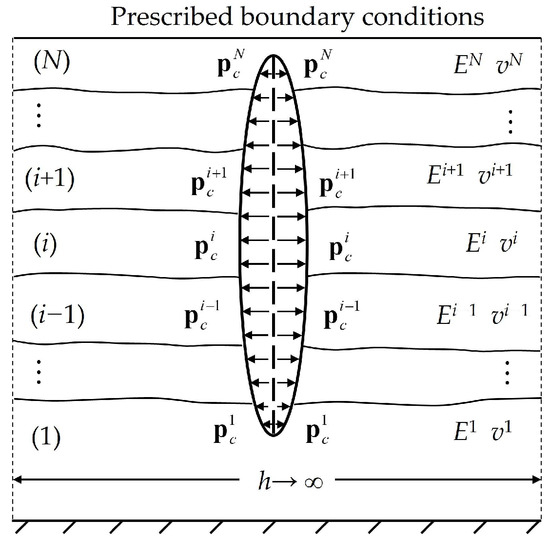
Figure 1. Schematic view of the crack problem [50].
The labeling in the figure follows the convention of the works authored by Maier and Novati [50]. The index (i) denotes the i-th layer and ranges from 1 (the bottom layer) to N (the top layer). The superscript i represents the material properties and quantities of interest (traction and displacement) associated with the i-th layer. The long dash line in the center implies the initial status of a slit-like crack characterized by two surfaces, one of which overlaps the other effectively. The two short dash lines at the two sides indicate the fictitious side boundaries, which are assumed in “undisturbed” regions and characterized by vanishing (zero) displacement, since the distance of them, h, is assumed to be infinite.
Matrices and column vectors are denoted by bold symbols. Thus, vectors of the nodal traction and displacement are indicated by p and u, respectively. The quantities pertaining to the lower (bottom), upper (top), side boundaries, and crack surfaces of each layer are denoted by the subscripts b, t, s, and c, respectively.
The boundary conditions of the multilayered system are usually of the type
ub1 = 0, ptN = p0
usi = 0 (1 ≤ i ≤ N)
As a result, the equations associated with the side boundaries can be split out of those pertaining to other boundaries [50].
The local coordinate defined in [41] is adopted in the paper, leading to the following interface continuity conditions.
uti = −ubi+1, pti = pbi+1
3. Displacement Discontinuity Method (DDM)
The DDM, proposed by Crouch [51], exploits the physical analog of a slit-like crack and a distribution of a series of constant displacement discontinuities or a distribution of a series of edge-dislocation dipoles (Figure 2). As a result, the DDM only focuses on the elements on the crack surface by discretizing it as a unity. In other words, it is not necessary for the DDM to introduce elements along interfaces, if any, while other numerical methods have to take care of the interfaces, making the DDM perhaps the most efficient numerical method for an analysis of the crack problems [37].
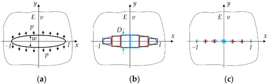
Figure 2. Physical analog of (a) a slit-like crack and (b) a distribution of a series of constant displacement discontinuities or (c) a distribution of a series of edge-dislocation dipoles.
3.1. Homogeneous Medium
The DDM was proposed under the assumption that (1) a crack lies in a homogeneous and isotropic medium and (2) equal loadings apply on the two crack surfaces (Figure 2a). The boundary-element equation of the DDM can be written in a concise form as
KD = p
where K is the coefficient matrix obtained from the DDM. Its explicit form is referred to in Ref. [51]. It is worth noting that the K obtained from the theory of constant displacement discontinuities and that obtained from the theory of edge dislocation are mathematically the same. D is the nodal opening displacement of the elements on the crack surface. p is the known nodal pressure on the crack surface. Thus, the crack opening displacement is
D = (K)−1p
In addition, the analytical solution to the crack problem in a homogeneous medium is given as the following [52][53]:
𝐷0=−4(1−𝑣2)𝐸𝑝𝑙2−𝑥2−−−−−−√
The percentage errors of the DDM with respect to the analytical solution with different numbers of the uniform crack element are illustrated in Figure 3, in which only the left-half part of the crack is displayed because of the symmetry. The abscissa is normalized by x/l, so that the coordinate −1 represents the crack tip. Figure 3b involves 100 crack elements, while only 11 elements are shown for visual simplicity.
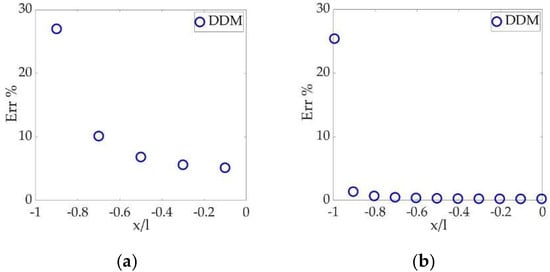
Figure 3. Percentage errors of the DDM with (a) 5 elements and (b) 100 elements.
Figure 3 demonstrates that a refined mesh leads to a more satisfying accuracy along the crack surface, except the tip, where the error of the DDM keeps around 26%.
3.2. The Higher-Order Tip-Element Approach
In order to improve the tip accuracy of the DDM, Shou and Crouch [54] developed the tip-element approach by replacing the constant displacement discontinuity (DD), also known as the zeroth-order element, at the tips with a higher-order quadratic DD (Figure 4). Constant DD is still assumed for elements other than at the tip, while the higher-order tip element assumes D~r1/2, where D is the opening displacement and r is the distance from a point in the tip element to its nearer tip point (x = −l for the left tip element and x = l for the right tip element). As a result, the approach captures the asymptotic behavior of the near-tip stress field due to the DD, leading to better tip accuracy.
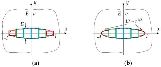
Figure 4. The DDM (a) without the tip-element approach and (b) with the tip-element approach.
The tip-element approach yields a boundary-element equation in the same form as Equation (4), while the explicit form of the K is referred to in Ref. [54]. The errors of the DDM with the tip element and the conventional DDM are displayed in Figure 5, which demonstrates significant improvement of the tip accuracy due to the higher-order tip element. The tip error decreases from around 26% to around 9%.
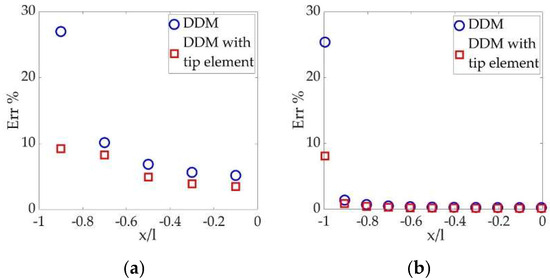
Figure 5. Percentage errors of the conventional DDM and the DDM with the tip element: (a) 5 crack elements and (b) 100 crack elements.
The tip-element approach, however, is restricted to the homogeneous medium. Once the media becomes inhomogeneous, the approach fails. In addition, some attempts have been made to place higher-order elements on the whole crack surface for even better accuracy [55][56]. Unfortunately, they are also limited to a homogeneous medium.
3.3. Two Bonded Half-Planes
Although the tip-element approach only applies to the homogeneous medium, the conventional DDM can be extended to the two bonded half-planes (Figure 6), since the Dundur’s equation that characterizes the stress field of an edge dislocation in the two bonded half-planes can be used as an analytical fundamental solution [52][57].
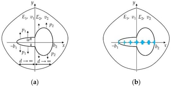
Figure 6. Physical analog of (a) a slit-like crack in two bonded half-planes and (b) a distribution of a series of edge-dislocation dipoles.
The DDM for the two bonded half-planes results in a boundary-element equation in the same form as Equation (4), while the explicit form of the K is based on the Dundur’s equation and can be referred to Refs. [52][57]. A semi-analytical solution to the crack problem in the two bonded half-planes is available with an additional continuity condition [58][59]:
1−𝑣21𝐸1𝑝1=1−𝑣22𝐸2𝑝2
The percentage error of the DDM with respect to the semi-analytical solution is shown in Figure 7. In the computation, the material properties are set as E1 = 3.07 (GPa), v1 = 0.35, E2 = 68.95 (GPa), and v2 = 0.3. The thickness of layer d is assumed to be 100 times of the larger one of b1 and b2, approximating the condition of the infinite d. In total, 10 uniform elements are placed on the shorter segment of the crack for a reasonably refined discretization.
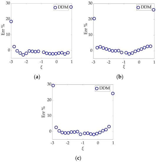
Figure 7. Percentage error of the DDM with b1/b2 = (a) 1/25; (b) 1/1; and (c) 2/1.
In Figure 7, the abscissa is normalized using
Thus, coordinate −3 and 1 represent the two crack tips. The result shows that the DDM matches well with the benchmark, except at the tip. Unfortunately, researchers cannot apply the tip-element approach here since the media becomes inhomogeneous.
3.4. Summary
The section has reviewed the DDM and its implementation for the crack problems in a homogeneous medium and two bonded half-planes. The method only requires elements on the crack surface and provides well-accepted accuracy, except at the tip. The tip-element approach improves the tip accuracy significantly, while it is not applicable to inhomogeneous media. In addition, the DDM is restricted in the cases of a homogeneous medium and two bonded half-planes since there are no existing analytical fundamental solutions to construct the boundary-element equations for the DDM in general multilayered media. Although some attempts [20][47][48] have been made to extend the DDM for general multilayered media, the extensions turn out to be first-order approximations, instead of full solutions [60][61].
4. Direct Method (DM)
Unlike the DDM that utilizes a physical analog of a slit-like crack and a distribution of a series of DDs or edge-dislocation dipoles, the traditional boundary-element method determines boundary-element equations directly by using the Kelvin’s solution and the reciprocal theorem [62][63][64][65][66]. Thus, the method is also known as the direct method (DM) [41]. The implementation of the DM for the multilayered media involves construction of a boundary-element equation for each layer and subsequent assembly of the equations with the continuity conditions along interfaces. Such a procedure usually generates an awfully large system of equations, of which all the unknowns are then solved simultaneously, undermining both accuracy and efficiency significantly [67]. Thus, it becomes necessary to decompose the large final system of equations into smaller ones by using the chain-like properties, i.e., the continuity conditions on the interfaces of the multilayered media [49][68]. Unfortunately, the DM cannot distinguish the effects of elements placed along one crack surface from those placed along the other surface. Thus, the DM cannot be applied to the crack problems directly [41]. The implementation of the DM for the multilayered media that does not contain cracks, however, inspires subsequent studies on the DM for the crack problems in multilayered media. As a result, researchers shall still review the DM here in a relatively concise manner.
4.1. Transfer Stiffness Method (TSM)
Maier and Novati [49] developed a method to decompose the final large system of a boundary-element equation into smaller ones. The method sets up the boundary-element equation for each layer of the multilayered media with the DM in the form
Hiui = pi
When the elements on the top and bottom surfaces are placed in pair (Figure 8a), Equation (10) can be rewritten to Equation (11) so that the quantities on the bottom interface can be expressed in terms of those on the top interfaces after some basic arrangements:
where Tuui = − (Htbi)−1Htti, Tupi = (Htbi)−1, Tpui = Hbti − Hbb(Htbi)−1Htti, and Tppi = Hbbi (Htbi)−1.
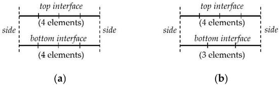
Figure 8. Elements on the top and bottom interfaces are placed (a) in pair and (b) not in pair.
Equation (11) can be written into a more concise form as
From Equation (12), researchers can solve the unknown displacements and tractions on the very top and bottom boundaries of the media using the chain-like property of the multilayered media, i.e., Equation (3), as a continuity condition on the interface:
Equation (13) is a recursive formula. When i = N, researchers can solve pb1 and utN, since ub1 and ptN are prescribed in Equation (1) as the boundary condition. Having obtained pb1 and utN, researchers can evaluate i from 2 to N−1 to obtain all the unknown displacements and tractions on the bottom and top interfaces of the layer that ranges from 2 to N−1. In other words, the TSM solves the unknowns by transferring the displacements and tractions on the bottom interface to those on the top interface of a layer with a sequential product of matrices from T1 to Ti.
Although the TSM manages to decompose the large final system of equations into smaller ones to improve efficiency, it suffers several computational issues that limit its application severely [45][50]:
- (1)
-
It requires elements on the top and bottom interfaces in pair;
- (2)
-
It categorizes the elements according to the type of unknown (displacement or traction). In practical applications, however, the displacement in mm and traction in kPa or MPa differs in magnitude of several orders. Therefore, an extra scaling that makes displacement and traction in the same order is necessary in case of ill-conditioning, undermining the efficiency of the method;
- (3)
-
It results in a highly ill-conditioned matrix H when dealing with a thick layer.
In order to address the issues above, Maier and Novati [50] proposed the successive stiffness method (SSM) that can be implemented in a more robust manner.
4.2. Successive Stiffness Method (SSM)
The SSM follows the same path of the TSM until Equation (10), from which the SSM derives a recursive formula [50]:
pti = Ĥttiuti
Ĥtt1 = Htt1
When i = 2~N,
Ĥtti = Htti − Htbi(Hbbi + Ĥtti−1)Hbti
Based on Equation (14), the SSM derived another two recursive formulae for i = 2~N:
ubi = [(Ĥtti−1 − Hbbi)−1Hbti]uti
pbi = Ĥtti−1uti
Having obtained Equations (14), (17) and (18), researchers can firstly obtain utN from Equation (14), since ptN is given as a boundary condition. Substitution of the solved utN into Equations (17) and (18) with i = N solves both ubN and pbN. The continuity condition on the interface gives utN−1 = −ubN and ptN−1 = pbN. Then, researchers can repeat the procedure to obtain ubN−1 and pbN−1 by replacing i = N by i = N − 1 in Equations (17) and (18). In such a recursive manner, researchers can compute all the unknowns successively from the very top layer to the very bottom one in a descending order, making the method quite convenient for numerical implementation. In addition, the method does not suffer the computational issues of the TSM.
4.3. Summary
The section has reviewed the DM and its implementation for multilayered media. The TSM decomposes the final large system of equations by utilizing the chain-like property (continuity condition on interfaces) of the media and categorizing the boundary element according to the type of unknown (displacement or traction). On the other hand, the SSM categorizes the boundary element by the categorization of the boundaries (bottom or top) and consequently overcomes the computational issues of the TSM. It is worth noting that neither the two methods are applicable for the crack problems directly, since the DM cannot distinguish the effects of elements placed along one crack surface from those placed along the other crack surface.
5. Consecutive Stiffness Method (CSM)
5.1. Pre-Treatment
The inapplicability of the DM to solve crack problems is attributed to the incapability of the DM to distinguish effects of the elements on the two overlapping crack surfaces [41]. If researchers divide the media artificially along the crack surface, however, the media will be divided into two subdomains with a pair of imaginary interfaces denoted by I and I’ (Figure 9). Then, researchers construct the boundary-element equation for each subdomain and assemble them with the continuity conditions on I and I’. The assembled equation turns out to be applicable to computing opening displacement of a slit-like crack [38][41].
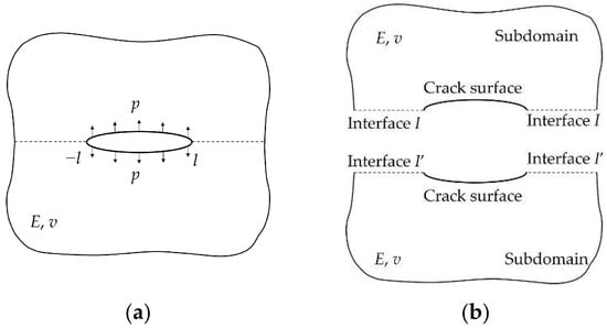
Figure 9. The artificial division: (a) division of the original media along the crack surface (dash line) and (b) the resultant subdomains and the imaginary interfaces I and I’.
researchers can now solve the crack problem in a homogeneous medium by dividing the medium in the way shown in Figure 9 and obtain the assembled boundary-element equation to compute the crack opening displacement. The details of the assembly and the consequent discretization can be referred to in Ref. [69]. The results obtained with the DM are compared to those obtained with the conventional DDM and the DDM with the tip element (Figure 10).
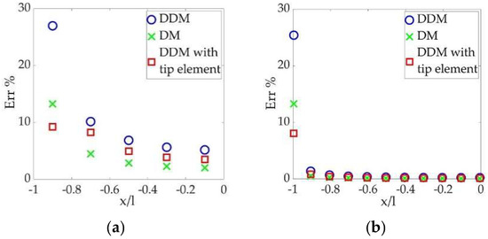
Figure 10. Percentage errors of the conventional DDM, the DM, and the DDM with tip element: (a) 5 crack elements and (b) 100 crack elements.
Figure 10 indicates that the DM shows the most satisfying accuracy except at the tip, since the integrals involved in the implementation of the DM can be evaluated analytically under the plane–strain condition [41]. Although the higher-order tip-element approach yields the best tip accuracy, the DM that uses the zeroth-order element can still obtain a comparable accuracy at the tip. On the other hand, the requirement of the pre-treatment makes the DM much slower than the DDM.
All the computations in the paper were conducted with MATLAB 2021a on a desktop with an Intel(R) Core (TM) i9-13900KF 3.00GHz CPU and 32GB RAM. Table 1 clearly indicates that the DM is much slower than the DDM, not only because of the pre-treatment but also due to the necessity to take care of the elements on the resultant interfaces I and I’, while the DDM only concentrates on the crack surface elements.
The pre-treatment shown in Figure 9 enables the application of the DM for crack problems in multilayered media. In Figure 11, the blue and red lines represent the two crack surfaces that effectively overlap each other, respectively. researchers cut the media along the crack surface (Figure 11a) artificially and acquire the resultant subdomains (Figure 11b). After that, researchers set up a boundary-element equation for each subdomain and assembled the equations with continuity conditions on all the interfaces.
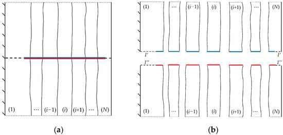
Figure 11. Pre-treatment of the DM for crack problems in multilayered media: (a) original configuration and (b) resultant configuration after the division.
It is obvious that an increase in the number of layers leads to a more cumbersome implementation, as researchers need to set up the boundary-element equation for each subdomain and assemble them all together. The procedure finally results in an extraordinarily huge system of equations, further deteriorating the efficiency of the DM. In order to improve the efficiency, Long et al. [69] proposed a consecutive stiffness method to break the huge system of equations into smaller ones and enable a recursive formula for faster computation by utilizing the chain-like property, i.e., the interfacial continuity condition of the media.
5.2. Formulations and Algorithm
The CSM divides the media and obtains the resultant subdomain in the way shown in Figure 11. After setting up a boundary-element equation for each subdomain, the CSM assembles two subdomains of a given layer through the resultant interface I’ and I’’, if any. If the given layer is an inner layer, e.g., the i-th layer in Figure 11b, the CSM simply patches the two systems of equations into one, since there is no resultant interface for the layer. Such a procedure eventually leads to a new system of equations for each layer, instead of a system of equations for the whole multilayered media. After that, the CSM derives recursive formulae to calculate unknowns for a faster computation by following the procedure of the SSM. In addition, the CSM derives a particular recursive formula that only focuses on the crack opening displacement uc so that all the other unknowns are eliminated during intermediate procedures, ensuring a further faster computation. Considering the limit of the page, researchers only present the four key equations of the method below. The detailed derivation of the equations is referred to in Ref. [69].
𝐮𝑡𝑁=(𝐇̂ 𝑡𝑡𝑁)−1𝐩𝑡𝑁−𝐂𝑁𝐩c𝑁−𝐆(𝑁)(𝑁−1)𝐩̂ 𝑡𝑁−1
𝐮𝑐𝑁=−(𝐇̃ 𝑐𝑐𝑁)−1[𝐇̃ 𝑐𝑡𝑁−𝐇̃ 𝑐𝑏𝑁(𝐀𝑁−𝐇̂ 𝑡𝑡1)−1𝐁𝑁]𝐮𝑡𝑁+(𝐇̃ 𝑐𝑐𝑁)−1{[𝑰−𝐇̃ 𝑐𝑏𝑁(𝐀𝑁−𝐇̂ 𝑡𝑡𝑁−1)−1𝐇̃ 𝑐𝑏𝑁(𝐇̃ 𝑐𝑐𝑁)−1]𝐩𝑐𝑁+𝐇̃ 𝑐𝑏𝑁(𝐀𝑁−𝐇̂ 𝑡𝑡𝑁−1)−1𝐩̂ 𝑡𝑁−1
𝐮𝑐𝑖−1=−(𝐇̃ 𝑐𝑡𝑖𝐇¯𝑡𝑡𝑖−1𝐇𝑡𝑐𝑖−1𝐇̃ 𝑐𝑐𝑖−1)−1𝐇̃ 𝑐𝑡𝑖−1[𝐇¯𝑏𝑐𝑖𝐮𝑐𝑖+𝐮̂ 𝑏𝑖+𝐇¯𝑡𝑡𝑖−1𝐇̃ 𝑡𝑐𝑖−1𝐩̃ 𝑐𝑖−1], 𝑖=2~𝑁
𝐮𝑐1=(𝐇̃ 𝑐𝑐1)−1[𝐩𝑐1+𝐇̃ 𝑐𝑡1𝐮𝑡1(𝐇¯𝑏𝑐2𝐮𝑐2+𝐮̂ 𝑏𝑖)]
Equation (21) is the particular recursive formula in which i ranges from 2 to N. In Equations (19)–(22), the matrices, such as Ĥ, 𝐇, H, A, C, etc., and the vectors at the right-hand side, such as pc, 𝐩̂ 𝑡, 𝐮̂ 𝑏, 𝐩̃ 𝑐, etc., are all known. The details of those quantities are available in Ref. [69]. Having obtained the four equations, researchers can conduct a sequential computation to solve the displacements on the crack surfaces consecutively in each layer in a descending order from the very top layer to the very bottom one. The flowchart of the computation is shown in Figure 12.
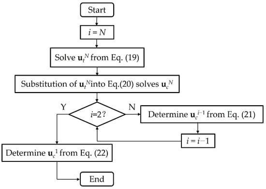
Figure 12. Flowchart of the computation to solve crack problems in multilayered media with the CSM.
The calculated displacement of a crack surface in all the layers uc contains two parts: the displacement of the upper crack surfaces, denoted by uc+, and that of the lower crack surfaces, denoted by uc−. According to the local coordinate used in the work, the crack opening displacement Dc is the following:
Dc = uc− + uc+
5.3. Numerical Examples
The discretization of the CSM is referred to in Ref. [69]. researchers compare the crack opening displacements obtained with the DDM and the CSM for the crack problem in two bonded half-planes (Figure 13).
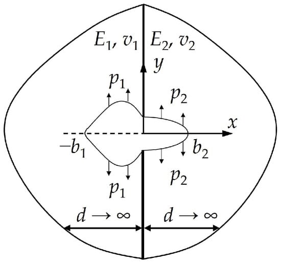
Figure 13. Schematic view of the crack problem in two bonded half-planes.
The parameters remain the same as in Section 3.3. The percentage errors of the DDM and the CSM are displayed in Figure 14.
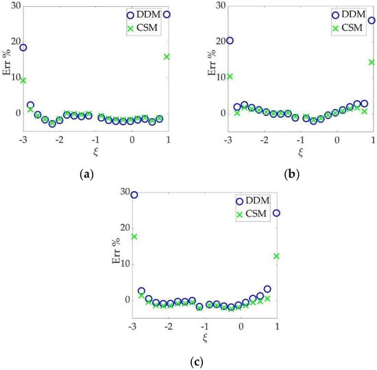
Figure 14. Percentage errors of the DDM and the CSM with b1/b2 = (a) 1/25; (b) 1/1; and (c) 2/1.
Figure 14 illustrates that both the DDM and the DM match the semi-analytical solution well along the crack surface, except at the tips. The CSM obtains tip errors that are lower than 20%, which is acceptable for practical engineering applications. Furthermore, the CSM leads to generally satisfactory results when the ratio of crack segments falls in the practical range, i.e., the value of b1/b2 falls in one order of magnitude.
5.4. Summary
The section has reviewed the CSM that implements the DM in a way that an artificial division of the multilayered media is made, enabling sequential computation to solve the displacements on the crack surfaces in each layer consecutively in a descending order from the very top layer to the very bottom one. Figure 10 and Figure 14 illustrate acceptable accuracy of the DM even with the zeroth-order element because analytical evaluation is available for the integrals involved in the DM under the plane–strain condition [41], indicating that the DM-based CSM can be used as a convincing benchmark to test other methods for crack problems in multilayered media. Furthermore, Table 1 and Table 2 have demonstrated the inefficiency of the CSM.
It is also worth noting that the inefficiency excludes the CSM for practical industrial applications, such as hydraulic-fracturing treatment that usually sets up the system of equations to conduct millions of time steps’ computation because of an excessively small time step for numerical stability [70][71][72][73]. For each time step, the newly introduced elements on the imaginary interfaces due to the artificial division result in a larger system of equations to manipulate [74][75][76], severely deteriorating the efficiency. In addition, when multiple cracks are involved, the CSM gets even slower and cumbersome for numerical implementation, since each crack requires an artificial division and consequent additional computation. Therefore, it is natural to conceive a method that shares both the efficiency of the DDM and broad applicability of the DM after the division.
6. Combined Boundary-Element Method
Ref. [19] incorporated the generalized Kelvin’s solution, the fundamental analytical solution of the DM, to the DDM with the Fourier transform, illustrating combination of the two methods from the aspect of basic theory. On the other hand, Ref. [13] attempts to extend the DDM with a “dividing and patch” approach, showing a simpler combination. Inspired by the two works, Long and Xu [77] presented a method that sets up the stiffness matrix of each layer with the DDM and characterizes the effects of the interfaces with the DM. Thus, the method that combines the DDM and the DM shares both the efficiency of the DDM and broad applicability of the DM after the artificial division.
6.1. Formulations and Algorithm
Figure 15 schematically illustrates a given (the i-th) layer after the deformation due to crack opening. The interfaces are sketched parallel for visual simplicity. Then, two artificial half-planes in the same material property marked in green and blue are patched with the layer on its original bottom and top interfaces (vertical dash lines), respectively.
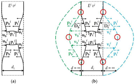
Figure 15. Schematic view of the artificial patch: (a) the i-th layer after the deformation and (b) the i-th layer patched with two half-planes in the same material property.
Having patched the two half-planes to the given layer, researchers apply tractions of the same magnitudes but in the opposite directions of the interfacial tractions. Thus, the interfaces of the two half-planes deform artificial nodal displacement vbi and vti, respectively (Figure 15b). The nodal displacement discontinuities on the two interfaces are
Dbi = ubi + vbi, Dti = uti + vti
In addition, the resultant medium becomes homogeneous, enabling implementation of the tip-element approach for the resultant artificial crack. Thus, researchers set up the matrix Ki for the elements at the crack tips marked by red circles in Figure 15b with the tip-element approach and construct Ki for the non-tip elements with the conventional DDM:
KiDi = pi
where the matrices Kcti, etc., are determined with the configuration of the i-th layer. Thus, they can be treated as known quantities.
On the other hand, researchers can also construct the boundary-element equation for the patched half-planes based on the DM:
Hbbivbi = pbi, Httivti = pti
Equations (25) and (27) are the starting point of the combined method. The method derives recursive formulae to obtain the final equation system that contains only the crack opening Dc for an even faster computation. Similar to the review of the CSM (Section 5.2), researchers only present the key equations of the combined method here, considering the limit of the page. The detailed explanation and derivation are referred to in Ref. [77].
When i = 1, the stiffness matrices of the combined method are
where the matrices 𝐊, etc., are resultant matrices after fundamental calculations of the basic matrices K, etc., and H, etc., in Equations (25) and (27).
𝐊̂ 𝑐𝑐1=𝐊̃ 𝑐𝑐1, 𝐊̂ 𝑐𝑡1=𝐊̃ 𝑐𝑡1, 𝐊̂ 𝑡𝑐1=𝐊̃ 𝑡𝑐1, 𝐊̂ 𝑡𝑡1=𝐊̃ 𝑡𝑡1
When i = 2~N, the stiffness matrices of the combined method are
𝐊̂ 𝑖𝑐𝑐=⎡⎣⎢⎢𝐊̂ 𝑖−1𝑐𝑐−𝐊̂ 𝑖−1𝑐𝑡(𝐐𝑖−1𝑏𝑏)−1𝐊̂ 𝑖−1𝑡𝑐𝐉𝑐𝑖−1𝑏𝑖𝐊𝑖𝑏𝑐𝐊𝑖𝑐𝑏 𝐍𝑖𝑏𝑏𝐊̂ 𝑖−1𝑡𝑐𝐊𝑖𝑐𝑐−𝐌𝑖𝑐𝑏𝐊𝑖𝑏𝑐⎤⎦⎥⎥, 𝐊̂ 𝑖𝑐𝑡=⎡⎣⎢𝐉𝑐𝑖−1𝑏𝑖𝐊𝑖𝑏𝑡 𝐊𝑖𝑐𝑡−𝐌𝑖𝑐𝑏𝐊𝑖𝑏𝑡⎤⎦⎥,𝐊̂ 𝑖𝑡𝑐=[𝐊𝑖𝑡𝑏 𝐍𝑖𝑏𝑏𝐊̂ 𝑖−1𝑡𝑐𝐊𝑖𝑡𝑐−𝐌𝑖𝑡𝑏𝐊𝑖𝑏𝑐], 𝐊̂ 𝑖𝑡𝑡=𝐊𝑖𝑡𝑡−𝐌𝑖𝑡𝑏𝐊𝑖𝑏𝑡
𝐃̂ 𝑐𝑁=[𝐊̂ 𝑐𝑐𝑁−𝐊̂ 𝑐𝑡𝑁(𝐊̂ 𝑡𝑡𝑁)−1𝐊̂ 𝑡𝑐𝑁]−1[𝐩̂ 𝑡𝑁−𝐊̂ 𝑐𝑡𝑁(𝐊̂ 𝑡𝑡𝑁)−1𝐩𝑡𝑁]
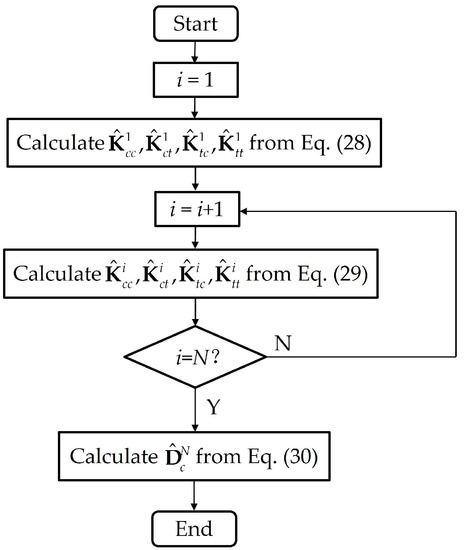
Figure 16. Flowchart of the computation to solve crack problems in multilayered media with the combined method.
6.2. Numerical Examples
6.2.1. Two Bonded Half-Planes
The discretization of the combined method is referred to in Ref. [77]. researchers firstly compare the percentage errors of the DDM, the CSM, and the combined method for the crack problem in the two bonded half-planes in Figure 17, while the parameters remain the same as in Section 3.3. The figure illustrates a satisfying match of the three methods to the semi-analytical solution, except at the tips. The combined method incorporated with the tip-element approach gives the best tip accuracy. Furthermore, it does not affect the results of the combined method significantly when the crack length ratio remains in the practical range (up to 25) in different materials.
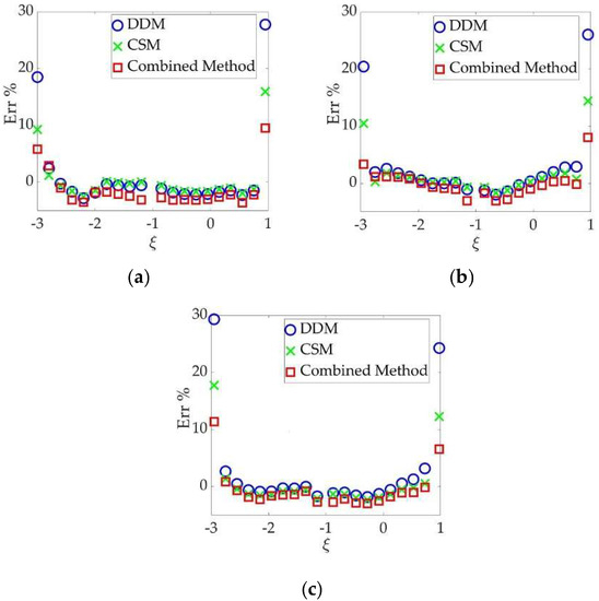
Figure 17. Percentage errors of the DDM, the CSM, and the combined method with b1/b2 = (a) 1/25; (b) 1/1; and (c) 2/1.
6.2.2. General Multilayered Media
The second example is calculation of crack opening in general multilayered media, in which the number of layers is more than three. researchers chose five-layered media, in which a crack intersects the parallel interfaces perpendicularly (Figure 18).
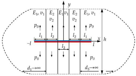
Figure 18. Schematic view of the crack problem in five-layered media.
researchers set the crack segment as l1 = 12l2. The Poisson ratios of the softer and stiffer layers are 0.25 and 0.3, respectively. The pressure p0 remains a known constant. The percentage difference of the crack opening displacement obtained using the combined method and that obtained using the CSM with a different Young’s modulus contrast and different numbers of the crack element on the thin layers are displayed from Figure 19, Figure 20 and Figure 21, in which only half of the results are shown due to the symmetry.
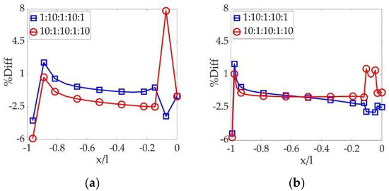
Figure 19. The difference of the combined method and the CSM with 10-fold E contrast: (a) 1 crack element on the thin layer and (b) 5 crack elements on the thin layer.
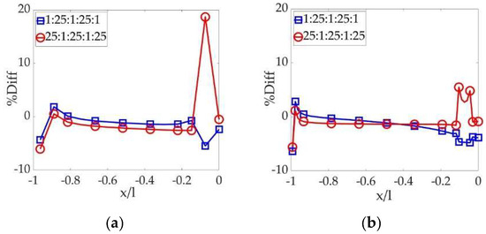
Figure 20. The difference of the combined method and the CSM with 25-fold E contrast: (a) 1 crack element on the thin layer and (b) 5 crack elements on the thin layer.
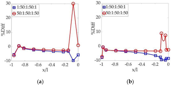
Figure 21. The difference of the combined method and the CSM with 50-fold E contrast: (a) 1 crack element on the thin layer and (b) 5 crack elements on the thin layer.
All of the three figures clearly illustrate a “peak” difference on the thin-and-softer layers neighbored by thick-and-stiffer ones. Fortunately, researchers can alleviate the “peak” difference by refining the discretization. In addition, higher E contrast results in a higher “peak” difference and requires more refined elements to mitigate it consequently. When the discretization is refined sufficiently, the results obtained with the two methods are quite close to each other.
6.2.3. Approximation of Thin-Layer Scaling
In practical hydraulic-fracturing treatments, a fluid-driven crack sometimes passes through a few thin layers sandwiched by thicker ones. Such thin layers usually require awfully refined discretization for accurate simulation, slowing down the computation significantly. It is well accepted that efficiency and accuracy are both critical factors for practical industrial applications. A satisfying numerical simulation in industry should keep a balance between the two factors, instead of sacrificing one to satisfy the other. Thus, the thin layers might be scaled as a single relatively thick layer with average effective material properties as in Equation (31) for better efficiency with the combined method:
where j is the index of the n thin layers, and lj is the thickness of the j-th layer. Thus, the original crack problem in Figure 18 is approximated with that in Figure 22.
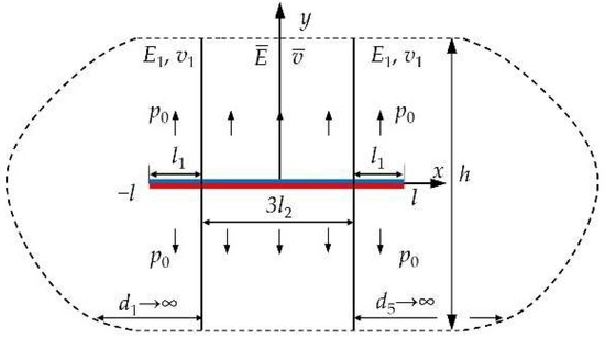
Figure 22. Schematic view of the crack problem in the approximated three-layered media.
The combined method placed only one crack element on the crack surface in the scaled layer characterized by Ē and v for even faster computation. The calculated crack opening displacement is then compared to that obtained using the combined method with coarse mesh (one element on the thin layer) in the original five-layered media and that obtained using the CSM with refined mesh (five elements on the thin layer) in the original five-layered media. As indicated previously, the results obtained using the CSM with refined mesh can be used as convincing benchmarks. The comparisons with different contrasts in Young’s modulus are shown from Figure 23, Figure 24 and Figure 25. In the three figures, the crack opening displacement w0 is normalized using
𝑤0=𝑤𝐺1𝑝0𝑙
where w is the crack opening displacement and G1 is the shear modulus of the first layer.
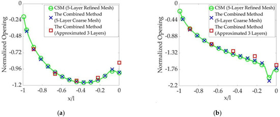
Figure 23. The crack openings obtained using the three methods with 10-fold E contrast: (a) E contrast 1:10:1:10:1 and (b) E contrast 10:1:10:1:10.
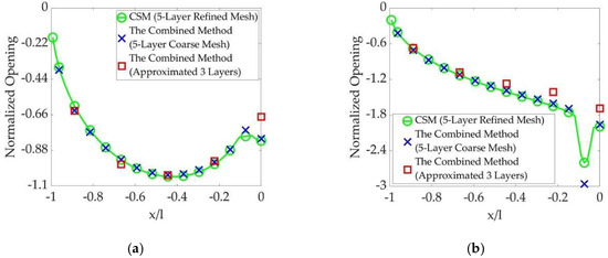
Figure 24. The crack openings obtained using the three methods with 25-fold E contrast: (a) E contrast 1:25:1:25:1 and (b) E contrast 25:1:25:1:25.
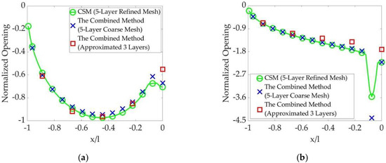
Figure 25. The crack openings obtained using the three methods with 50-fold E contrast: (a) E contrast 1:50:1:50:1 and (b) E contrast 50:1:50:1:50.
The three figures validate the approximation of the thin-layer scaling for more efficient computation when the contrast in Young’s modulus remains up to 10-fold, since the approximated crack opening obtained using the combined method differs from the original crack opening obtained using the CSM with refined mesh by less than 20% (Figure 23).
When the contrast in Young’s modulus gets higher, the original crack opening obtained using the CSM with refined mesh on the thin-and-soft layers neighbored by a thick-and-hard one reaches about twice of the approximated opening calculated using the combined method (Figure 24b and Figure 25b). On the other hand, it is interesting to find the approximation to be valid for a contrast in Young’s modulus up to 50-fold when a thin-and-stiff layer is neighbored by thick-and-soft ones (Figure 24a and Figure 25a).
6.3. Summary
The section has reviewed the combined method that constructs the stiffness matrix of each layer with the DDM and characterizes the effects of the interfaces with the DM. As a result, the method shares both the efficiency of the DDM and broad applicability of the DM after the division, as demonstrated in the numerical examples. In addition, the final system of equations only contains unknown crack opening displacements, leading to even faster computation. The combined method has also adopted the tip-element approach, ensuring a well-acceptable accuracy including at the tips, while the tip accuracy cannot be improved with refined discretization only. The numerical examples also validated an approximation of thin-layer scaling with the combined method under practical conditions for a more-efficient industrial simulation, for example, hydraulic-fracturing simulation. The crack intersects interface(s), if any, perpendicularly in the numerical examples, since some analytical or semi-analytical solutions are available in such conditions. In fact, the combined method can deal with more-complicated crack patterns, such as crack inclining to interfaces. Examples of using the method to simulate propagation of practical hydraulic fractures can be found in Refs. [12][75][78].
References
- Xiao, H.; Yue, Z. Elastic fields in two joined transversely isotropic media of infinite extent as a result of rectangular loading. Int. J. Numer. Anal. Methods Geomech. 2013, 37, 247–277.
- Xie, Y.; Xiao, H.; Yue, Z. The behavior of vertically non-homogeneous elastic solids under internal rectangular loads. Eur. J. Environ. Civ. Eng. 2022, 26, 1936–1961.
- Xiao, B.; Fang, J.; Long, G.; Tao, Y.; Huang, Z. Analysis of thermal conductivity of damaged tree-like bifurcation network withfractal roughened surfaces. Fractals 2022, 30, 2250104.
- Zhang, Y.; Xiao, B.; Tu, B.; Zhang, G.; Wang, Y.; Long, G. Fractal analysis for thermal conductivity of dual porous media embedded with asymmetric tree-like bifurcation networks. Fractals 2023, 31, 2350046.
- Hamzah, K.; Long, N.; Senu, N.; Eshkuvatov, K. Numerical solution for crack phenomenon in dissimilar materials under various mechanical loadings. Symmetry 2021, 13, 235.
- Liang, M.; Liu, Y.; Xiao, B.; Yang, S.; Wang, Z. An analytical model for the transverse permeability of gas diffusion layer with electrical double layer effects in proton exchange membrane fuel cells. Int. J. Hydrogen Energy 2018, 43, 17880–17888.
- Xiao, B.; Huang, Q.; Chen, H.; Chen, X.; Long, G. A fractal model for capillary flow through a single tortuous capillary with roughened surfaces in fibrous porous media. Fractals 2021, 29, 2150017.
- An, S.; Zou, H.; Li, W.; Deng, Z. Experimental investigation on the vibration attenuation of tensegrity prisms integrated with particle dampers. Acta Mech. Solida Sin. 2022, 35, 672–681.
- Gao, J.; Xiao, B.; Tu, B.; Chen, F.; Liu, Y. A fractal model for gas diffusion in dry and wet fibrous media with tortuous converging-diverging capillary bundle. Fractals 2022, 30, 2250176.
- Liu, S.; Valko, P.; McKetta, S.; Liu, X. Microseismic closure window characterizes hydraulic-fracture geometry better. SPE Reserv. Eval. Eng. 2017, 20, 423–445.
- Adachi, J.; Siebrits, E.; Peirce, A.; Desroches, J. Computer simulation of hydraulic fractures. Int. J. Rock Mech. Min. Sci. 2007, 44, 739–757.
- Long, G.; Liu, S.; Xu, G.; Wong, S.; Chen, H.; Xiao, B. A perforation-erosion model for hydraulic-fracturing applications. SPE Prod. Oper. 2018, 33, 770–783.
- Shen, B.; Stephansson, O.; Rinne, M. Modelling Rock Fracturing Processes: A Fracture Mechanics Approach Using FRACOD; Springer: London, UK, 2014.
- Cui, C.; Zhang, Q.; Banerjee, U.; Babuška, I. Stable generalized finite element method (SGFEM) for three-dimensional crack problems. Numer. Math. 2022, 152, 475–509.
- Liu, S.; Valko, P. A rigorous hydraulic-fracture equilibrium-height model for multilayer formations. SPE Prod. Oper. 2018, 33, 214–234.
- Xiao, B.; Zhu, H.; Chen, F.; Long, G.; Li, Y. A fractal analytical model for Kozeny-Carman constant and permeability of roughened porous media composed of particles and converging-diverging capillaries. Powder Technol. 2023, 420, 118256.
- Cheng, W.; Jiang, G.; Xie, J.; Wei, Z.; Zhou, Z.; Li, X. A simulation study comparing the Texas two-step and the multistage consecutive fracturing method. Pet. Sci. 2019, 16, 1121–1133.
- Xiao, H.; Yue, Z.; Zhao, X. A generalized Kelvin solution based method for analyzing elastic fields in heterogeneous rocks due to reservoir water impoundment. Comput. Geosci. 2012, 43, 126–136.
- Xiao, H.; Yue, Z. A three-dimensional displacement discontinuity method for crack problems in layered rocks. Int. J. Rock Mech. Min. Sci. 2011, 48, 412–420.
- Hirose, S.; Sharma, M. Numerical Modelling of Fractures in Multilayered Rock Formations Using a Displacement Discontinuity Method. In In Proceedings of the 52nd U.S. Rock Mechanics/Geomechanics Symposium, Seattle, WA, USA, 17–20 June 2018.
- Zeng, Q.; Bo, L.; Liu, W.; Huang, Z.; Yao, J. An investigation of hydraulic fracture propagation in multi-layered formation via the phase field method. Comput. Geotech. 2023, 156, 105258.
- Zhu, D.; Zhang, L.; Song, X.; Lian, H.; Niu, D. Propagation mechanism of the hydraulic fracture in layered-fractured-plastic formations. Int. J. Fract. 2023, 241, 189–210.
- Xiao, B.; Wang, P.; Wu, J.; Zhu, H.; Liu, M.; Liu, Y.; Long, G. A novel fractal model for gas diffusion coefficient in dry porous media embedded with a damaged tree-like branching network. Fractals 2022, 30, 2250150.
- Alizadeh, R.; Marji, M.; Abdollahipour, A.; Sagand, M. Numerical simulation of fatigue crack propagation in heterogeneous geomaterials under varied loads using displacement discontinuity method. J. Rock Mech. Geotech. Eng. 2023, 15, 702–716.
- Zhuang, X.; Li, X.; Zhou, S. Transverse penny-shaped hydraulic fracture propagation in naturally-layered rocks under stress boundaries: A 3D phase field modeling. Comput. Geotech. 2023, 155, 105205.
- Zhang, G.; Guo, T.; Elkhodary, K.; Tang, S.; Guo, X. Mixed Graph-FEM phase field modeling of fracture in plates and shells with nonlinearly elastic solids. Comput. Methods Appl. Mech. Eng. 2022, 389, 114282.
- Li, P.; Li, W.; Li, B.; Yang, S.; Shen, Y.; Wang, Q.; Zhou, K. A review on phase field models for fracture and fatigue. Eng. Fract. Mech. 2023, 289, 109419.
- Zhang, G.; Qiu, H.; Elkhodary, K.; Tang, S.; Peng, D. Modeling tunable fracture in hydrogel shell structures for biomedical applications. Gels 2022, 8, 515.
- Chen, L. Phase-Field Modelling of Material Microstructure. Multiscale Materials Modelling Fundamentals and Applications; Woodhead Publishing: Sawston, UK, 2007; pp. 62–83.
- Zhang, G.; Guo, T.; Guo, X.; Tang, S.; Flemming, M.; Liu, W. Fracture in tension-compression-asymmetry solids via phase field modeling. Comput. Methods Appl. Mech. Eng. 2019, 357, 112573.
- Zhang, G.; Tang, C.; Chen, P.; Long, G.; Cao, J.; Tang, S. Advancements in phase-field modeling for fracture in nonlinear elastic solids under finite deformations. Mathematics 2023, 11, 3366.
- Zhang, Q.; Cui, C.; Banerjee, U.; Babuška, I. A condensed generalized finite element method (CGFEM) for interface problems. Comput. Methods Appl. Mech. Eng. 2022, 391, 114537.
- Ambati, M.; Gerasimov, T.; De Lorenzis, L. A review on phase-field models of brittle fracture and a new fast hybrid formulation. Comput. Mech. 2015, 55, 383–405.
- Cheng, W.; Jin, Y.; Chen, M.; Jiang, G. Numerical stress analysis for the multi-casing structure inside a wellbore in the formation using the boundary element method. Pet. Sci. 2017, 14, 126–137.
- Wang, P.; Xiao, B.; Gao, J.; Zhu, H.; Liu, M.; Long, G.; Li, P. A novel fractal model for spontaneous imbibition in damaged tree-like branching networks. Fractals 2023, 31, 2350010.
- Cheng, W.; Lu, C.; Feng, G.; Xiao, B. Ball sealer tracking and seating of temporary plugging fracturing technology in the perforated casing of a horizontal well. Energy Explor. Exploit. 2021, 39, 2045–2061.
- Peirce, A.; Siebrits, E. Uniform asymptotic approximations for accurate modeling of cracks in layered elastic media. Int. J. Fract. 2001, 110, 205–239.
- Blandford, G.; Ingraffea, A.; Liggett, J. Two-dimensional stress intensity factor computations using the boundary element method. Int. J. Numer. Methods Eng. 1981, 17, 387–404.
- Detournay, E.; Gordeliy, E. Displacement discontinuity method for modeling axisymmetric cracks in an elastic half-space. Int. J. Solids Struct. 2011, 48, 2614–2629.
- Yue, Z.; Xiao, H. Generalized Kelvin solution based boundary element method for crack problems in multilayered solids. Eng. Anal. Bound. Elem. 2002, 26, 691–705.
- Crouch, S.; Starfield, A. Boundary Element Methods in Solid Mechanics; George Allen & Unwein: London, UK, 1983.
- Thompson, W. Transmission of elastic waves through a stratified medium. J. Appl. Phys. 1950, 21, 89–93.
- Gilbert, F.; Backus, G. Propagator matrices in elastic wave and vibration problems. Geophysics 1966, 31, 326–332.
- Buffler, H. Theory of elasticity of a multilayered medium. J. Elast. 1971, 1, 125–143.
- Peirce, A.; Siebrits, E. The scaled flexibility matrix method for the efficient solution of boundary value problems in 2D and 3D layered elastic media. Comput. Methods Appl. Mech. Eng. 2001, 190, 5935–5956.
- Benitez, F.; Rosakis, A. Three-dimensional elastostatics of a layer and a layered medium. J. Elast. 1987, 18, 3–50.
- Shou, K.; Napier, J. A two-dimensional linear variation displacement discontinuity method for three-layered elastic media. Int. J. Rock Mech. Min. Sci. 1999, 36, 719–729.
- Shou, K. A superposition scheme to obtain fundamental boundary element solutions in multi-layered elastic media. Int. J. Numer. Anal. Methods Geomech. 2000, 24, 795–814.
- Maier, G.; Novati, G. On boundary element-transfer matrix analysis of layered elastic systems. Eng. Anal. 1986, 3, 208–216.
- Maier, G.; Novati, G. Boundary element elastic analysis of layered soils by a successive stiffness method. Int. J. Numer. Anal. Methods Geomech. 1987, 11, 435–447.
- Crouch, S. Solution of plane elasticity problems by the displacement discontinuity method. Int. J. Numer. Methods Eng. 1976, 10, 301–343.
- Asaro, R.; Lubarda, V. Mechanics of Solids and Materials; Cambridge University Press: New York, NY, USA, 2006.
- Yan, X. An effective boundary element method for analysis of crack problems in a plane elastic plate. Appl. Math. Mech. 2005, 26, 814–822.
- Shou, K.; Crouch, S. A higher order displacement discontinuity method for analysis of crack problems. Int. J. Rock Mech. Min. Sci. Geomech. Abstr. 1995, 32, 49–55.
- Shou, K.; Siebrits, E.; Crouch, S. A higher-order displacement discontinuity method for three-dimensional elastostatic problems. Int. J. Rock Mech. Min. Sci. 1997, 34, 317–322.
- Li, J.; Liu, Y.; Wu, K. A new higher-order displacement discontinuity method based on the joint element for analysis of close-spacing planar fractures. SPE J. 2022, 27, 1123–1139.
- Dundurs, J. Elastic Interactions of Dislocations with Inhomogeneities; ASME: New York, NY, USA, 1969; pp. 70–115.
- Erdogan, F.; Biricikoglu, V. Two bonded half planes with a crack going through the interface. Int. J. Eng. Sci. 1973, 11, 745–766.
- Cook, L.; Erdogan, F. Stresses in bonded materials with a crack perpendicular to the interface. Int. J. Eng. Sci. 1972, 10, 677–697.
- Siebrits, E.; Crouch, S. On the paper “A two-dimensional linear variation displacement discontinuity method for three-layered elastic media” by Keh-Jian Shou and J.A.L. Napier, International Journal of Rock Mechanics and Mining Sciences, Vol. 36(6), 719-729, 1999. Int. J. Rock Mech. Min. Sci. 2000, 37, 873–875.
- Shou, K.; Napier, J. Author’s reply to discussion by E. Siebrits and S. L. Crouch regarding the paper ‘A two-dimensional linear variation displacement discontinuity method for three-layered elastic media’, Keh-Jian Shou and J.A.L. Napier, International Journal of Rock Mechanics and Mining Sciences, Vol. 36(6), 719–729, 1999. Int. J. Rock Mech. Min. Sci. 2000, 37, 877–878.
- Nowak, P.; Hall, J. Direct boundary element method for dynamics in a half-space. Bull. Seismol. Soc. Am. 1993, 83, 1373–1390.
- Segond, D.; Tafreshi, A. Stress analysis of three-dimensional contact problems using the boundary element method. Eng. Anal. Bound. Elem. 1998, 22, 199–214.
- Tsinopoulos, S.; Kattis, S.; Polyzos, D.; Beskos, D. An advanced boundary element method for axisymmetric elastodynamic analysis. Comput. Methods Appl. Mech. Eng. 1999, 175, 53–70.
- Oliveria, M.; Dumont, N.; Selvadurai, A. Boundary element formulation of axisymmetric problems for an elastic halfspace. Eng. Anal. Bound. Elem. 2012, 36, 1478–1492.
- Hattori, G.; Alatawi, I.; Trevelyan, J. An extended boundary element method for formulation for the direct calculation of the stress intensity factors in fully anisotropic materials. Int. J. Numer. Anal. Methods Geomech. 2017, 109, 965–981.
- Linkov, A.; Fillipov, N. Difference equations approach to the analysis of layered systems. Meccanica 1991, 26, 195–209.
- Siebrits, E.; Peirce, A. An efficient multi-layer planar 3D fracture growth algorithm using a fixed mesh approach. Int. J. Numer. Methods Eng. 2002, 53, 691–717.
- Long, G.; Liu, Y.; Xu, W.; Zhou, P.; Zhou, J.; Xu, G.; Xiao, B. Analysis of crack problems in multilayered elastic medium by a consecutive stiffness method. Mathematics 2022, 10, 4403.
- Cheng, W.; Jiang, G.; Zhou, Z.; Wei, Z.; Li, X. Numerical simulation for the dynamic breakout of a borehole using boundary element method. Geotech. Geol. Eng. 2019, 38, 2873–2881.
- Al Hameli, F.; Suboyin, A.; Al Kobaisi, M.; Rahman, M.; Haroun, M. Modeling fracture propagation in a dual-porosity system: Pseudo-3D-carter-dual-porosity model. Energies 2022, 15, 6779.
- Donstov, E. Analysis of a constant height hydraulic fracture driven by a power-law fluid. Rock Mech. Bull. 2022, 1, 100003.
- Luo, T.; Liu, S.; Liu, S. A productivity model for vertical wells with horizontal multi-fractures. Int. J. Oil Gas Coal Technol. 2022, 31, 225–241.
- Cheng, H.; Detournay, A. A direct boundary element method for plane strain poroelasticity. Int. J. Numer. Anal. Methods Geomech. 1988, 12, 551–572.
- Zhai, Z.; Fonseca, E.; Azad, A.; Cox, B. A new tool for multi-cluster & multi-well hydraulic fracture modeling. In Proceedings of the SPE Hydraulic Fracturing Technology Conference, Woodlands, TX, USA, 3–5 February 2015.
- Munoz, L.; Mejia, C.; Rueda, J.; Roehl, D. Pseudo-coupled hydraulic fracturing analysis with displacement discontinuity and finite element methods. Eng. Fract. Mech. 2022, 274, 108774.
- Long, G.; Xu, G. A combined boundary integral method for analysis of crack problems in multilayered elastic media. Int. J. Appl. Mech. 2016, 8, 1650070.
- Long, G.; Xu, G. The effects of perforation erosion on practical hydraulic-fracturing applications. SPE J. 2017, 22, 645–659.
More
Information
Contributors
MDPI registered users' name will be linked to their SciProfiles pages. To register with us, please refer to https://encyclopedia.pub/register
:
View Times:
568
Revisions:
2 times
(View History)
Update Date:
19 Oct 2023
Table of Contents


Notice
You are not a member of the advisory board for this topic. If you want to update advisory board member profile, please contact office@encyclopedia.pub.
OK
Confirm
Only members of the Encyclopedia advisory board for this topic are allowed to note entries. Would you like to become an advisory board member of the Encyclopedia?
Yes
No
${ textCharacter }/${ maxCharacter }
Submit
Cancel
Back
Comments
${ item }
|
${ item.createdUser.fullName }
${ item.createdAt }
${ item.vote }
${ item.reply }
Delete
${ reply.createdUser.fullName }
${ reply.createdAt }
${ reply.vote }
Delete
There is no reply to this comment~
${ item.replyTextCharacter }/${ item.replyMaxCharacter }
Submit
Cancel
More
No more~
There is no comment~
${ textCharacter }/${ maxCharacter }
Submit
Cancel
${ selectedItem.replyTextCharacter }/${ selectedItem.replyMaxCharacter }
Submit
Cancel
Confirm
Are you sure to Delete?
Yes
No